Computer vision e CNN
In questo capitolo tratteremo la computer vision e le reti convoluzionali.
In generale in Pytorch per scaricare le immagini si utilizzata la libreria "torchvision" le cui specifiche sono dettagliate nella pagina di documentazione datasets
Inizieremo ad utilizzare Fashion-MNIST che contiene immagini di vestiti vedi fashion-ds
Per caricare il dataset di immagini basterà utilizzare la specifiica libreria utilizzato il metodo che ne porta il nome come sotto riportato:
train_data = datasets.FashionMNIST(root='data', # dove scaricare le immagini
                                   train=True, # si vogliono anche le immagini di training
                                   download=True, #si vogliono scaricare
                                   transform=torchvision.transforms.ToTensor(), # tvogliamo trasformare le immagini in tensori
                                   target_transform=None # le immagini di test non verranno convertite in tensori
                                   )
dopo aver carico le immgini di training vediamone una:
Di seguito un esempio di modello lineare:
@get_time
def training_model_0(device):

    # creiamo il modello
    class FashionMNISTModelV0(nn.Module):
        def __init__(self, input_shape: int, hidden_units: int, output_shape: int):
            super().__init__()
            self.layer_stack = nn.Sequential(
                nn.Flatten(),  # neural networks like their inputs in vector form
                nn.Linear(in_features=input_shape, out_features=hidden_units),
                nn.ReLU(),
                # in_features = number of features in a data sample (784 pixels)
                nn.Linear(in_features=hidden_units, out_features=output_shape),
                nn.ReLU(),
            )

        def forward(self, x):
            return self.layer_stack(x)

    # Need to setup model with input parameters
    model_0 = FashionMNISTModelV0(input_shape=28 * 28,  # one for every pixel (28x28)
                                  hidden_units=10,  # how many units in the hiden layer
                                  output_shape=len(class_names)  # one for every class
                                  )
    model_0.to(device)  # keep model on CPU to begin with

    # Setup loss function and optimizer
    loss_fn = nn.CrossEntropyLoss()  # this is also called "criterion"/"cost function" in some places
    optimizer = torch.optim.SGD(params=model_0.parameters(), lr=0.1)

    # Set the number of epochs (we'll keep this small for faster training times)
    epochs = 3

    # Create training and testing loop
    for epoch in tqdm(range(epochs)):
        print(f"Epoch: {epoch}\n-------")
        ### Training
        train_loss = 0
        # Add a loop to loop through training batches
        for batch, (X, y) in enumerate(train_dataloader):
            model_0.train()

            y = y.to(device)
            X = X.to(device)

            # 1. Forward pass
            y_pred = model_0(X)

            # 2. Calculate loss (per batch)
            loss = loss_fn(y_pred, y)
            train_loss += loss  # accumulatively add up the loss per epoch

            # 3. Optimizer zero grad
            optimizer.zero_grad()

            # 4. Loss backward
            loss.backward()

            # 5. Optimizer step
            optimizer.step()

            # Print out how many samples have been seen
            if batch % 400 == 0:
                print(f"Looked at {batch * len(X)}/{len(train_dataloader.dataset)} samples")

        # Divide total train loss by length of train dataloader (average loss per batch per epoch)
        train_loss /= len(train_dataloader)

        ### Testing
        # Setup variables for accumulatively adding up loss and accuracy
        test_loss, test_acc = 0, 0
        model_0.eval()
        with torch.inference_mode():
            for X, y in test_dataloader:
                y = y.to(device)
                X = X.to(device)

                # 1. Forward pass
                test_pred = model_0(X)

                # 2. Calculate loss (accumatively)
                test_loss += loss_fn(test_pred, y)  # accumulatively add up the loss per epoch

                # 3. Calculate accuracy (preds need to be same as y_true)
                test_acc += accuracy_fn(y_true=y, y_pred=test_pred.argmax(dim=1))

            # Calculations on test metrics need to happen inside torch.inference_mode()
            # Divide total test loss by length of test dataloader (per batch)
            test_loss /= len(test_dataloader)

            # Divide total accuracy by length of test dataloader (per batch)
            test_acc /= len(test_dataloader)

        ## Print out what's happening
        print(f"\nTrain loss: {train_loss:.5f} | Test loss: {test_loss:.5f}, Test acc: {test_acc:.2f}%\n")

    return model_0
ora, utilizzando un modello lineare non si ottengono risultati eccellenti, per la gestione della computer vision è meglio utilizzare una rete convoluzionale che fa uso per es. di layer Conv2D e MaxPool2D come sotto riportato:

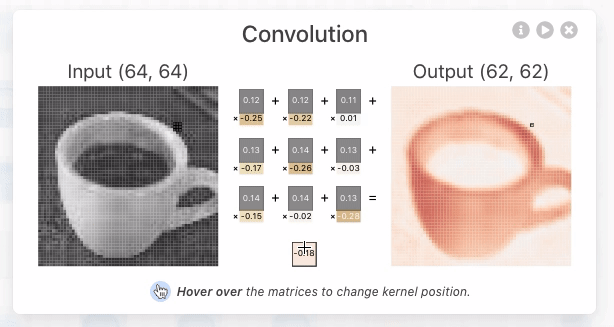
Il layer Conv2D si occupa di trovare e evidenziare le caratteristiche più importanti dell'immagine passata in input, mediante uno scaling dell'immagine stessa applicando dei pesi a ciascun tensore che associato al pixel dell'immagine.
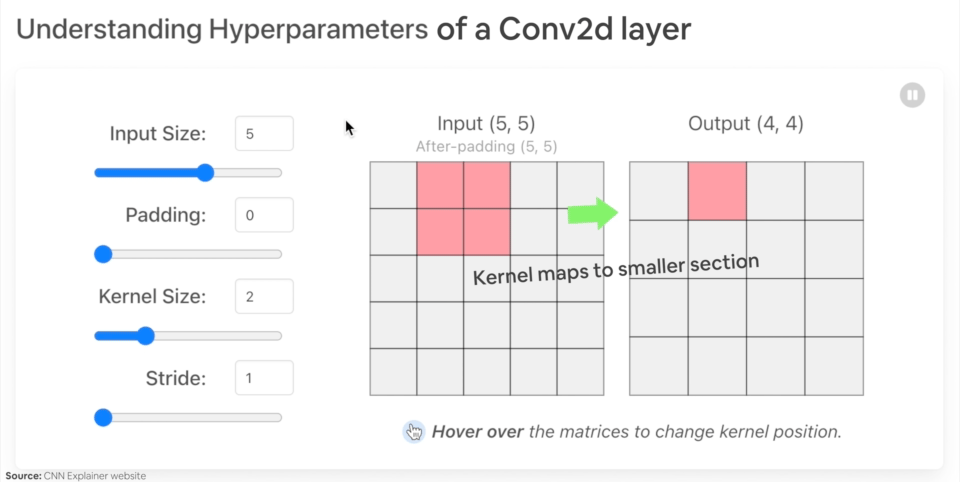
Il MaxPool2D invece scala l'imagine selezionando il tensore con valore maggiore all'interno dei un'area della matrice dei tensori.
Di seguito un esempio di rete convoluzionale in pytorch:
import torch
from torch import nn
from torch.utils.data import DataLoader
import torchvision
from torchvision import datasets
from torchvision import transforms
from torchvision.transforms import ToTensor
# Import tqdm for progress bar
from tqdm.auto import tqdm
import matplotlib.pylab as plt
from src.formazione.utils.utilita import get_time
# carichiamo le immagini
train_data = datasets.FashionMNIST(root='data', # dove scaricare le immagini
train=True, # si vogliono anche le immagini di training
download=True, #si vogliono scaricare
transform=torchvision.transforms.ToTensor(), # tvogliamo trasformare le immagini in tensori
target_transform=None # le immagini di test non verranno convertite in tensori
)
test_data = datasets.FashionMNIST(root='data', # dove scaricare le immagini
train=False, # si vogliono anche le immagini di training
download=True, #si vogliono scaricare
transform=ToTensor(), # tvogliamo trasformare le immagini in tensori
target_transform=None # le immagini di test non verranno convertite in tensori
)
# nomi dei tipi di vestiti
class_names = train_data.classes
# Setup the batch size hyperparameter
BATCH_SIZE = 32
# Turn datasets into iterables (batches)
train_dataloader = DataLoader(train_data, # dataset to turn into iterable
batch_size=BATCH_SIZE, # how many samples per batch?
# num_workers =10,
shuffle=True # shuffle data every epoch?
)
test_dataloader = DataLoader(test_data,
batch_size=BATCH_SIZE,
shuffle=False # don't necessarily have to shuffle the testing data
)
def accuracy_fn(y_true, y_pred):
correct = torch.eq(y_true, y_pred).sum().item() # torch.eq() calculates where two tensors are equal
acc = (correct / len(y_pred)) * 100
return acc
# Set the seed and start the timer
torch.manual_seed(42)
@get_time
def training_model_0(device):
# creiamo il modello
class FashionMNISTModelV0(nn.Module):
def __init__(self, input_shape: int, hidden_units: int, output_shape: int):
super().__init__()
self.layer_stack = nn.Sequential(
nn.Flatten(), # neural networks like their inputs in vector form
nn.Linear(in_features=input_shape, out_features=hidden_units),
nn.ReLU(),
# in_features = number of features in a data sample (784 pixels)
nn.Linear(in_features=hidden_units, out_features=output_shape),
nn.ReLU(),
)
def forward(self, x):
return self.layer_stack(x)
# Need to setup model with input parameters
model_0 = FashionMNISTModelV0(input_shape=28 * 28, # one for every pixel (28x28)
hidden_units=10, # how many units in the hiden layer
output_shape=len(class_names) # one for every class
)
model_0.to(device) # keep model on CPU to begin with
# Setup loss function and optimizer
loss_fn = nn.CrossEntropyLoss() # this is also called "criterion"/"cost function" in some places
optimizer = torch.optim.SGD(params=model_0.parameters(), lr=0.1)
# Set the number of epochs (we'll keep this small for faster training times)
epochs = 3
# Create training and testing loop
for epoch in tqdm(range(epochs)):
print(f"Epoch: {epoch}\n-------")
### Training
train_loss = 0
# Add a loop to loop through training batches
for batch, (X, y) in enumerate(train_dataloader):
model_0.train()
y = y.to(device)
X = X.to(device)
# 1. Forward pass
y_pred = model_0(X)
# 2. Calculate loss (per batch)
loss = loss_fn(y_pred, y)
train_loss += loss # accumulatively add up the loss per epoch
# 3. Optimizer zero grad
optimizer.zero_grad()
# 4. Loss backward
loss.backward()
# 5. Optimizer step
optimizer.step()
# Print out how many samples have been seen
# if batch % 400 == 0:
# print(f"Looked at {batch * len(X)}/{len(train_dataloader.dataset)} samples")
# Divide total train loss by length of train dataloader (average loss per batch per epoch)
train_loss /= len(train_dataloader)
### Testing
# Setup variables for accumulatively adding up loss and accuracy
test_loss, test_acc = 0, 0
model_0.eval()
with torch.inference_mode():
for X, y in test_dataloader:
y = y.to(device)
X = X.to(device)
# 1. Forward pass
test_pred = model_0(X)
# 2. Calculate loss (accumatively)
test_loss += loss_fn(test_pred, y) # accumulatively add up the loss per epoch
# 3. Calculate accuracy (preds need to be same as y_true)
test_acc += accuracy_fn(y_true=y, y_pred=test_pred.argmax(dim=1))
# Calculations on test metrics need to happen inside torch.inference_mode()
# Divide total test loss by length of test dataloader (per batch)
test_loss /= len(test_dataloader)
# Divide total accuracy by length of test dataloader (per batch)
test_acc /= len(test_dataloader)
## Print out what's happening
print(f"\nTrain loss: {train_loss:.5f} | Test loss: {test_loss:.5f}, Test acc: {test_acc:.2f}%\n")
return model_0
@get_time
def training_model_2(device, epochs):
# creiamo il modello
class FashionMNISTModelV2(nn.Module):
"""
Questo modello utilizza una rete convuluzionale
"""
def __init__(self, input_shape: int, hidden_units: int, output_shape: int):
super().__init__()
padding = 1
self.con_block1 = nn.Sequential(
nn.Conv2d(in_channels=input_shape,out_channels=hidden_units, kernel_size=3, stride=1, padding=padding),
nn.ReLU(),
nn.Conv2d(in_channels=hidden_units, out_channels=hidden_units, kernel_size=3, stride=1, padding=padding),
nn.ReLU(),
nn.MaxPool2d(kernel_size=2) # prende il valore massimo dell'input portandolo in output, in pratica comprime l'input
)
self.con_block2 = nn.Sequential(
nn.Conv2d(in_channels=hidden_units ,out_channels=hidden_units, kernel_size=3, stride=1, padding=padding),
nn.ReLU(),
nn.Conv2d(in_channels=hidden_units, out_channels=hidden_units, kernel_size=3, stride=1, padding=padding),
nn.ReLU(),
nn.MaxPool2d(kernel_size=2) # prende il valore massimo dell'input portandolo in output, in pratica comprime l'input
)
self.classifier = nn.Sequential(
nn.Flatten(), # neural networks like their inputs in vector form
nn.Linear(in_features=hidden_units*7*7, out_features=hidden_units), # trucco per definire il numero di input features dopo un flatten è quello di visuallizare l'output del layer precedente
# in_features = number of features in a data sample (784 pixels)
nn.ReLU(),
nn.Linear(in_features=hidden_units, out_features=output_shape),
)
def forward(self, x):
x = self.con_block1(x)
# print(x.shape)
x = self.con_block2(x)
# print(x.shape)
x = self.classifier(x)
return x
# Need to setup model with input parameters
model_2 = FashionMNISTModelV2(
input_shape=1,
hidden_units=10, # how many units in the hiden layer
output_shape=len(class_names) # one for every class
)
model_2.to(device) # keep model on CPU to begin with
# Setup loss function and optimizer
loss_fn = nn.CrossEntropyLoss() # this is also called "criterion"/"cost function" in some places
optimizer = torch.optim.SGD(params=model_2.parameters(), lr=0.1)
# Create training and testing loop
for epoch in tqdm(range(epochs)):
# print(f"Epoch: {epoch}\n-------")
### Training
train_loss = 0
# Add a loop to loop through training batches
for batch, (X, y) in enumerate(train_dataloader):
model_2.train()
y = y.to(device)
X = X.to(device)
# 1. Forward pass
y_pred = model_2(X)
# 2. Calculate loss (per batch)
loss = loss_fn(y_pred, y)
train_loss += loss # accumulatively add up the loss per epoch
# 3. Optimizer zero grad
optimizer.zero_grad()
# 4. Loss backward
loss.backward()
# 5. Optimizer step
optimizer.step()
# Print out how many samples have been seen
# if batch % 400 == 0:
# print(f"Looked at {batch * len(X)}/{len(train_dataloader.dataset)} samples")
# Divide total train loss by length of train dataloader (average loss per batch per epoch)
train_loss /= len(train_dataloader)
### Testing
# Setup variables for accumulatively adding up loss and accuracy
test_loss, test_acc = 0, 0
model_2.eval()
with torch.inference_mode():
for X, y in test_dataloader:
y = y.to(device)
X = X.to(device)
# 1. Forward pass
test_pred = model_2(X)
# 2. Calculate loss (accumatively)
test_loss += loss_fn(test_pred, y) # accumulatively add up the loss per epoch
# 3. Calculate accuracy (preds need to be same as y_true)
test_acc += accuracy_fn(y_true=y, y_pred=test_pred.argmax(dim=1))
# Calculations on test metrics need to happen inside torch.inference_mode()
# Divide total test loss by length of test dataloader (per batch)
test_loss /= len(test_dataloader)
# Divide total accuracy by length of test dataloader (per batch)
test_acc /= len(test_dataloader)
## Print out what's happening
print(f"\nEpoch {epoch} Train loss: {train_loss:.5f} | Test loss: {test_loss:.5f}, Test acc: {test_acc:.2f}%\n")
return model_2
if __name__ == '__main__':
# training_model_0("cuda")
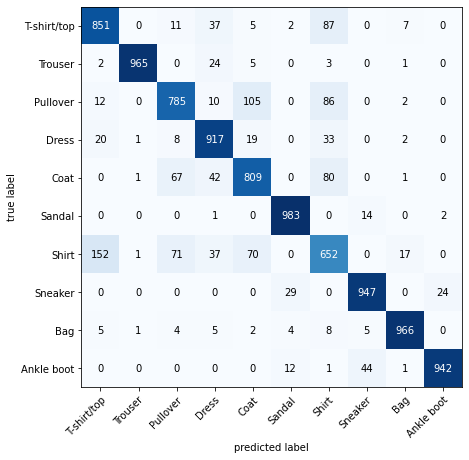
training_model_2("cuda", epochs=20)Confusion Matrix
from torchmetrics import ConfusionMatrix
from mlxtend.plotting import plot_confusion_matrix

# 2. Setup confusion matrix instance and compare predictions to targets
confmat = ConfusionMatrix(num_classes=len(class_names), task='multiclass')
confmat_tensor = confmat(preds=y_pred_tensor,
                         target=test_data.targets)

# 3. Plot the confusion matrix
fig, ax = plot_confusion_matrix(
    conf_mat=confmat_tensor.numpy(), # matplotlib likes working with NumPy
    class_names=class_names, # turn the row and column labels into class names
    figsize=(10, 7)
);