# Computer vision e CNN
In questo capitolo tratteremo la computer vision e le reti convoluzionali.
In generale in Pytorch per scaricare le immagini si utilizzata la libreria "torchvision" le cui specifiche sono dettagliate nella pagina di documentazione [datasets](https://pytorch.org/vision/stable/datasets.html)
Inizieremo ad utilizzare Fashion-MNIST che contiene immagini di vestiti vedi [fashion-ds](https://github.com/zalandoresearch/fashion-mnist)
Per caricare il dataset di immagini basterà utilizzare la specifiica libreria utilizzato il metodo che ne porta il nome come sotto riportato:
```python
train_data = datasets.FashionMNIST(root='data', # dove scaricare le immagini
train=True, # si vogliono anche le immagini di training
download=True, #si vogliono scaricare
transform=torchvision.transforms.ToTensor(), # tvogliamo trasformare le immagini in tensori
target_transform=None # le immagini di test non verranno convertite in tensori
)
```
dopo aver carico le immgini di training vediamone una:
image, label = train_data[0]
e otterremo:
[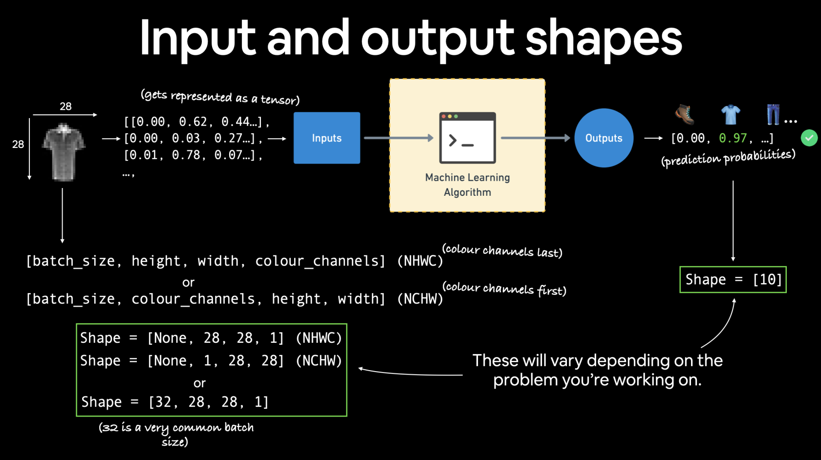](https://cms.marcocucchi.it/uploads/images/gallery/2023-05/5VcgpfIEYJBaRBMC-03-computer-vision-input-and-output-shapes.png)
Di seguito un esempio di modello lineare:
```python
@get_time
def training_model_0(device):
# creiamo il modello
class FashionMNISTModelV0(nn.Module):
def __init__(self, input_shape: int, hidden_units: int, output_shape: int):
super().__init__()
self.layer_stack = nn.Sequential(
nn.Flatten(), # neural networks like their inputs in vector form
nn.Linear(in_features=input_shape, out_features=hidden_units),
nn.ReLU(),
# in_features = number of features in a data sample (784 pixels)
nn.Linear(in_features=hidden_units, out_features=output_shape),
nn.ReLU(),
)
def forward(self, x):
return self.layer_stack(x)
# Need to setup model with input parameters
model_0 = FashionMNISTModelV0(input_shape=28 * 28, # one for every pixel (28x28)
hidden_units=10, # how many units in the hiden layer
output_shape=len(class_names) # one for every class
)
model_0.to(device) # keep model on CPU to begin with
# Setup loss function and optimizer
loss_fn = nn.CrossEntropyLoss() # this is also called "criterion"/"cost function" in some places
optimizer = torch.optim.SGD(params=model_0.parameters(), lr=0.1)
# Set the number of epochs (we'll keep this small for faster training times)
epochs = 3
# Create training and testing loop
for epoch in tqdm(range(epochs)):
print(f"Epoch: {epoch}\n-------")
### Training
train_loss = 0
# Add a loop to loop through training batches
for batch, (X, y) in enumerate(train_dataloader):
model_0.train()
y = y.to(device)
X = X.to(device)
# 1. Forward pass
y_pred = model_0(X)
# 2. Calculate loss (per batch)
loss = loss_fn(y_pred, y)
train_loss += loss # accumulatively add up the loss per epoch
# 3. Optimizer zero grad
optimizer.zero_grad()
# 4. Loss backward
loss.backward()
# 5. Optimizer step
optimizer.step()
# Print out how many samples have been seen
if batch % 400 == 0:
print(f"Looked at {batch * len(X)}/{len(train_dataloader.dataset)} samples")
# Divide total train loss by length of train dataloader (average loss per batch per epoch)
train_loss /= len(train_dataloader)
### Testing
# Setup variables for accumulatively adding up loss and accuracy
test_loss, test_acc = 0, 0
model_0.eval()
with torch.inference_mode():
for X, y in test_dataloader:
y = y.to(device)
X = X.to(device)
# 1. Forward pass
test_pred = model_0(X)
# 2. Calculate loss (accumatively)
test_loss += loss_fn(test_pred, y) # accumulatively add up the loss per epoch
# 3. Calculate accuracy (preds need to be same as y_true)
test_acc += accuracy_fn(y_true=y, y_pred=test_pred.argmax(dim=1))
# Calculations on test metrics need to happen inside torch.inference_mode()
# Divide total test loss by length of test dataloader (per batch)
test_loss /= len(test_dataloader)
# Divide total accuracy by length of test dataloader (per batch)
test_acc /= len(test_dataloader)
## Print out what's happening
print(f"\nTrain loss: {train_loss:.5f} | Test loss: {test_loss:.5f}, Test acc: {test_acc:.2f}%\n")
return model_0
```
ora, utilizzando un modello lineare non si ottengono risultati eccellenti, per la gestione della computer vision è meglio utilizzare una rete convoluzionale che fa uso per es. di layer Conv2D e MaxPool2D come sotto riportato:
[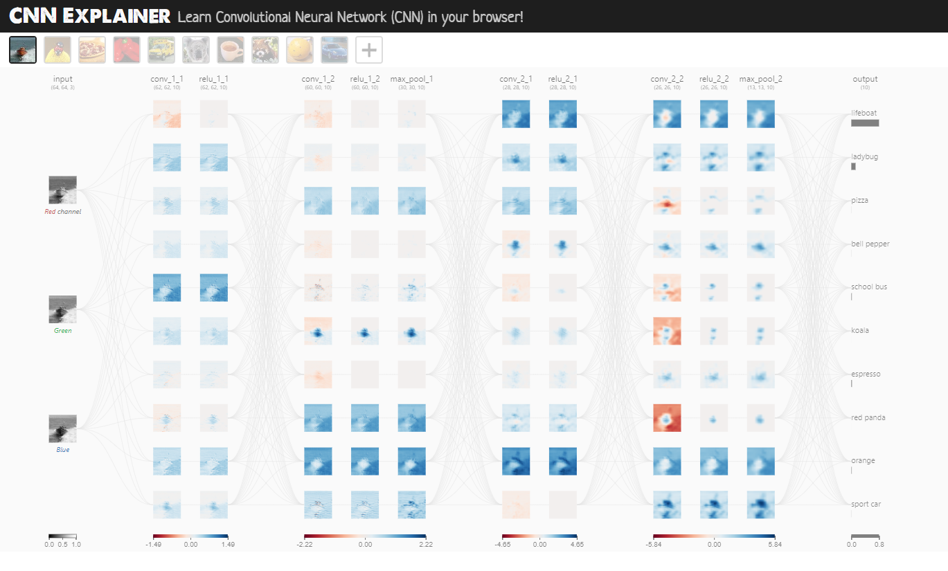](https://poloclub.github.io/cnn-explainer/)
Il layer Conv2D si occupa di trovare e evidenziare le caratteristiche più importanti dell'immagine passata in input, mediante uno scaling dell'immagine stessa applicando dei pesi a ciascun tensore che associato al pixel dell'immagine.
[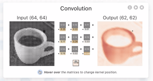](https://poloclub.github.io/cnn-explainer/ "rete convulazionale")
[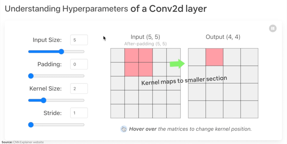](https://cms.marcocucchi.it/uploads/images/gallery/2023-06/ennEys0jJLIu7C76-image.png)
Il MaxPool2D invece scala l'imagine selezionando il tensore con valore maggiore all'interno dei un'area della matrice dei tensori.
Di seguito un esempio di rete convoluzionale in pytorch:
```python
import torch
from torch import nn
from torch.utils.data import DataLoader
import torchvision
from torchvision import datasets
from torchvision import transforms
from torchvision.transforms import ToTensor
# Import tqdm for progress bar
from tqdm.auto import tqdm
import matplotlib.pylab as plt
from src.formazione.utils.utilita import get_time
# carichiamo le immagini
train_data = datasets.FashionMNIST(root='data', # dove scaricare le immagini
train=True, # si vogliono anche le immagini di training
download=True, #si vogliono scaricare
transform=torchvision.transforms.ToTensor(), # tvogliamo trasformare le immagini in tensori
target_transform=None # le immagini di test non verranno convertite in tensori
)
test_data = datasets.FashionMNIST(root='data', # dove scaricare le immagini
train=False, # si vogliono anche le immagini di training
download=True, #si vogliono scaricare
transform=ToTensor(), # tvogliamo trasformare le immagini in tensori
target_transform=None # le immagini di test non verranno convertite in tensori
)
# nomi dei tipi di vestiti
class_names = train_data.classes
# Setup the batch size hyperparameter
BATCH_SIZE = 32
# Turn datasets into iterables (batches)
train_dataloader = DataLoader(train_data, # dataset to turn into iterable
batch_size=BATCH_SIZE, # how many samples per batch?
# num_workers =10,
shuffle=True # shuffle data every epoch?
)
test_dataloader = DataLoader(test_data,
batch_size=BATCH_SIZE,
shuffle=False # don't necessarily have to shuffle the testing data
)
def accuracy_fn(y_true, y_pred):
correct = torch.eq(y_true, y_pred).sum().item() # torch.eq() calculates where two tensors are equal
acc = (correct / len(y_pred)) * 100
return acc
# Set the seed and start the timer
torch.manual_seed(42)
@get_time
def training_model_0(device):
# creiamo il modello
class FashionMNISTModelV0(nn.Module):
def __init__(self, input_shape: int, hidden_units: int, output_shape: int):
super().__init__()
self.layer_stack = nn.Sequential(
nn.Flatten(), # neural networks like their inputs in vector form
nn.Linear(in_features=input_shape, out_features=hidden_units),
nn.ReLU(),
# in_features = number of features in a data sample (784 pixels)
nn.Linear(in_features=hidden_units, out_features=output_shape),
nn.ReLU(),
)
def forward(self, x):
return self.layer_stack(x)
# Need to setup model with input parameters
model_0 = FashionMNISTModelV0(input_shape=28 * 28, # one for every pixel (28x28)
hidden_units=10, # how many units in the hiden layer
output_shape=len(class_names) # one for every class
)
model_0.to(device) # keep model on CPU to begin with
# Setup loss function and optimizer
loss_fn = nn.CrossEntropyLoss() # this is also called "criterion"/"cost function" in some places
optimizer = torch.optim.SGD(params=model_0.parameters(), lr=0.1)
# Set the number of epochs (we'll keep this small for faster training times)
epochs = 3
# Create training and testing loop
for epoch in tqdm(range(epochs)):
print(f"Epoch: {epoch}\n-------")
### Training
train_loss = 0
# Add a loop to loop through training batches
for batch, (X, y) in enumerate(train_dataloader):
model_0.train()
y = y.to(device)
X = X.to(device)
# 1. Forward pass
y_pred = model_0(X)
# 2. Calculate loss (per batch)
loss = loss_fn(y_pred, y)
train_loss += loss # accumulatively add up the loss per epoch
# 3. Optimizer zero grad
optimizer.zero_grad()
# 4. Loss backward
loss.backward()
# 5. Optimizer step
optimizer.step()
# Print out how many samples have been seen
# if batch % 400 == 0:
# print(f"Looked at {batch * len(X)}/{len(train_dataloader.dataset)} samples")
# Divide total train loss by length of train dataloader (average loss per batch per epoch)
train_loss /= len(train_dataloader)
### Testing
# Setup variables for accumulatively adding up loss and accuracy
test_loss, test_acc = 0, 0
model_0.eval()
with torch.inference_mode():
for X, y in test_dataloader:
y = y.to(device)
X = X.to(device)
# 1. Forward pass
test_pred = model_0(X)
# 2. Calculate loss (accumatively)
test_loss += loss_fn(test_pred, y) # accumulatively add up the loss per epoch
# 3. Calculate accuracy (preds need to be same as y_true)
test_acc += accuracy_fn(y_true=y, y_pred=test_pred.argmax(dim=1))
# Calculations on test metrics need to happen inside torch.inference_mode()
# Divide total test loss by length of test dataloader (per batch)
test_loss /= len(test_dataloader)
# Divide total accuracy by length of test dataloader (per batch)
test_acc /= len(test_dataloader)
## Print out what's happening
print(f"\nTrain loss: {train_loss:.5f} | Test loss: {test_loss:.5f}, Test acc: {test_acc:.2f}%\n")
return model_0
@get_time
def training_model_2(device, epochs):
# creiamo il modello
class FashionMNISTModelV2(nn.Module):
"""
Questo modello utilizza una rete convuluzionale
"""
def __init__(self, input_shape: int, hidden_units: int, output_shape: int):
super().__init__()
padding = 1
self.con_block1 = nn.Sequential(
nn.Conv2d(in_channels=input_shape,out_channels=hidden_units, kernel_size=3, stride=1, padding=padding),
nn.ReLU(),
nn.Conv2d(in_channels=hidden_units, out_channels=hidden_units, kernel_size=3, stride=1, padding=padding),
nn.ReLU(),
nn.MaxPool2d(kernel_size=2) # prende il valore massimo dell'input portandolo in output, in pratica comprime l'input
)
self.con_block2 = nn.Sequential(
nn.Conv2d(in_channels=hidden_units ,out_channels=hidden_units, kernel_size=3, stride=1, padding=padding),
nn.ReLU(),
nn.Conv2d(in_channels=hidden_units, out_channels=hidden_units, kernel_size=3, stride=1, padding=padding),
nn.ReLU(),
nn.MaxPool2d(kernel_size=2) # prende il valore massimo dell'input portandolo in output, in pratica comprime l'input
)
self.classifier = nn.Sequential(
nn.Flatten(), # neural networks like their inputs in vector form
nn.Linear(in_features=hidden_units*7*7, out_features=hidden_units), # trucco per definire il numero di input features dopo un flatten è quello di visuallizare l'output del layer precedente
# in_features = number of features in a data sample (784 pixels)
nn.ReLU(),
nn.Linear(in_features=hidden_units, out_features=output_shape),
)
def forward(self, x):
x = self.con_block1(x)
# print(x.shape)
x = self.con_block2(x)
# print(x.shape)
x = self.classifier(x)
return x
# Need to setup model with input parameters
model_2 = FashionMNISTModelV2(
input_shape=1,
hidden_units=10, # how many units in the hiden layer
output_shape=len(class_names) # one for every class
)
model_2.to(device) # keep model on CPU to begin with
# Setup loss function and optimizer
loss_fn = nn.CrossEntropyLoss() # this is also called "criterion"/"cost function" in some places
optimizer = torch.optim.SGD(params=model_2.parameters(), lr=0.1)
# Create training and testing loop
for epoch in tqdm(range(epochs)):
# print(f"Epoch: {epoch}\n-------")
### Training
train_loss = 0
# Add a loop to loop through training batches
for batch, (X, y) in enumerate(train_dataloader):
model_2.train()
y = y.to(device)
X = X.to(device)
# 1. Forward pass
y_pred = model_2(X)
# 2. Calculate loss (per batch)
loss = loss_fn(y_pred, y)
train_loss += loss # accumulatively add up the loss per epoch
# 3. Optimizer zero grad
optimizer.zero_grad()
# 4. Loss backward
loss.backward()
# 5. Optimizer step
optimizer.step()
# Print out how many samples have been seen
# if batch % 400 == 0:
# print(f"Looked at {batch * len(X)}/{len(train_dataloader.dataset)} samples")
# Divide total train loss by length of train dataloader (average loss per batch per epoch)
train_loss /= len(train_dataloader)
### Testing
# Setup variables for accumulatively adding up loss and accuracy
test_loss, test_acc = 0, 0
model_2.eval()
with torch.inference_mode():
for X, y in test_dataloader:
y = y.to(device)
X = X.to(device)
# 1. Forward pass
test_pred = model_2(X)
# 2. Calculate loss (accumatively)
test_loss += loss_fn(test_pred, y) # accumulatively add up the loss per epoch
# 3. Calculate accuracy (preds need to be same as y_true)
test_acc += accuracy_fn(y_true=y, y_pred=test_pred.argmax(dim=1))
# Calculations on test metrics need to happen inside torch.inference_mode()
# Divide total test loss by length of test dataloader (per batch)
test_loss /= len(test_dataloader)
# Divide total accuracy by length of test dataloader (per batch)
test_acc /= len(test_dataloader)
## Print out what's happening
print(f"\nEpoch {epoch} Train loss: {train_loss:.5f} | Test loss: {test_loss:.5f}, Test acc: {test_acc:.2f}%\n")
return model_2
if __name__ == '__main__':
# training_model_0("cuda")
training_model_2("cuda", epochs=20)
```
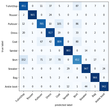
Confusion Matrix
```python
from torchmetrics import ConfusionMatrix
from mlxtend.plotting import plot_confusion_matrix
# 2. Setup confusion matrix instance and compare predictions to targets
confmat = ConfusionMatrix(num_classes=len(class_names), task='multiclass')
confmat_tensor = confmat(preds=y_pred_tensor,
target=test_data.targets)
# 3. Plot the confusion matrix
fig, ax = plot_confusion_matrix(
conf_mat=confmat_tensor.numpy(), # matplotlib likes working with NumPy
class_names=class_names, # turn the row and column labels into class names
figsize=(10, 7)
);
```
[](https://cms.marcocucchi.it/uploads/images/gallery/2023-06/x510sJWDunFBhbIc-image.png)