Multiclass classification
Nella classificazione multipla, a differenza della classificazione binaria possono essere identificate più di due categorie. Importante è comprendere l'utulizzo delle activation functions. Per la multiclass possiamo utilizzare la ReLU o la Sigmoid.
Per esempio voglio classificare 4 classi di "blobs" :) lol come nell'immagine sotto riportata, utilizzando il pacchetto sklearn:
from sklearn.datasets import make_blobs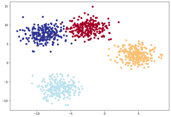
Il modello
costruisco il modello per la gestione della classificazione multipla:
class BlobModel(nn.Module): # la nn.Module è la superclasse da derivare per costruire un modello

# customizzo gli input al costruttore
def __init__(self, input_features, output_features, hidden_units=8):
"""Initializes all required hyperparameters for a multi-class classification model.

Args:
input_features (int): Number of input features to the model.
out_features (int): Number of output features of the model
(how many classes there are).
hidden_units (int): Number of hidden units between layers, default 8.
"""
super().__init__()

# definisco i layers e il numero di neuroni che li compongnono.
# NB: i layer sono lineari e quindi rispondono all'equazione y = xw+b

self.linear_layer_stack = nn.Sequential(
  nn.Linear(in_features=input_features, out_features=hidden_units),
  nn.ReLU(), # <- does our dataset require non-linear layers? (try uncommenting and see if the results change)
  nn.Linear(in_features=hidden_units, out_features=hidden_units),
  nn.ReLU(), # <- does our dataset require non-linear layers? (try uncommenting and see if the results change)
  nn.Linear(in_features=hidden_units, out_features=output_features), # how many classes are there?
)

def forward(self, x):
  return self.linear_layer_stack(x)
Da notare che l'ultimo livello della rete neurale, (l'output level) è composto da tanti neuroni quante sono le classi da classificare. Ciascun neurone di output è associato ad una classe e ne rappresenta la probabilità che l'intput appartenga ad a Niesima classe.
NB: ricordo che i livelli sono "lineari", il che significa che corrispondono all'equazione y=x⋅WeightsT+bias il che significa bisogna aggiungere delle funzioni non lineari in grado di "spezzare" le equazioni lineari. Potremmo inserire, tra un livello lineare e l'altro una funzion non lineare come la ReLU.
Ovvimante se i dati sono nettamente separati e quindi una linea retta li può "dividere" allora potremmo evitare di inserire le funzioni di attivazione non lineare. Nell'esempio sopra visabile i 4 gruppi di "blobs" possono essere appunto separati da linee rette, il modello potrà quindi anche (opzionale) non utilizzare le ReLU non lineari.
Per le funzioni di attivazione non lienari vedi:
La loss function
Per la classificazione multiclasse andiamo a vedere cosa pytorch offre nella pagina Loss functions
Per la binary classification in genere si usa la nn.BCEWithLogitsLoss mentre per la multiclassification si usa la nn.CrossEntropyLoss
TIP: Per la CrossEntropy fare attenzione al parametro "weight " da valorizzare nel caso i cui il numero di elementi delle classi sono diversi tra di loro, es. i gialli sono 100 metre i versi sono 20...
loss_fn = nn.CrossEntropyLoss()L'Optimizer
Come ottimizer possiamo utilizzare quelli generici come l'Adam o il pià classico SGD, vedi pagina optimezers.
optimizer = torch.optim.SGD(model_4.parameters(), lr=0.1)Il training loop
# Fit the model
torch.manual_seed(42)

# Set number of epochs
epochs = 100

# looppo..
for epoch in range(epochs):
  ### Training
  model_4.train()

  # 1. Forward pass
  y_logits = model_4(X_blob_train) # model outputs raw logits
  y_pred = torch.softmax(y_logits, dim=1).argmax(dim=1) # go from logits -> prediction probabilities -> prediction labels
  # print(y_logits)

  # 2. Calculate loss and accuracy
  loss = loss_fn(y_logits, y_blob_train)
  acc = accuracy_fn(y_true=y_blob_train,
  y_pred=y_pred)

  # 3. Optimizer zero grad
  optimizer.zero_grad()

  # 4. Loss backwards
  loss.backward()

  # 5. Optimizer step
  optimizer.step()

  ### Testing
  model_4.eval()
  with torch.inference_mode():
    # 1. Forward pass
    test_logits = model_4(X_blob_test)

    # NB: i logits vengono passati alla funzione softmax che restituisce la probabilità
    #     che un valore del vettori si verifichi... (un po' forzato ma spero renda l'idea)
    test_pred = torch.softmax(test_logits, dim=1).argmax(dim=1)

    # 2. Calculate test loss and accuracy
    test_loss = loss_fn(test_logits, y_blob_test)
    test_acc = accuracy_fn(y_true=y_blob_test,
    y_pred=test_pred)

    # Print out what's happening
    if epoch % 10 == 0:
      print(f"Epoch: {epoch} | Loss: {loss:.5f}, Acc: {acc:.2f}% | Test Loss: {test_loss:.5f}, Test Acc: {test_acc:.2f}%")
Importante capire il funzionamento della softmax alla quale verranno passati i logits. Per comprendere meglio la softmax vedi link.
La classe completa:
# Import dependencies
import torch
import matplotlib.pyplot as plt
from sklearn.datasets import make_blobs
from sklearn.model_selection import train_test_split
from torch import nn
import numpy as np

# Set the hyperparameters for data creation
NUM_CLASSES = 4
NUM_FEATURES = 2
RANDOM_SEED = 42

# 1. Create multi-class data
X_blob, y_blob = make_blobs(n_samples=1000,
                            n_features=NUM_FEATURES, # X features
                            centers=NUM_CLASSES, # y labels
                            cluster_std=1.5, # give the clusters a little shake up (try changing this to 1.0, the default)
                            random_state=RANDOM_SEED
                            )

# 2. Turn data into tensors
X_blob = torch.from_numpy(X_blob).type(torch.float)
y_blob = torch.from_numpy(y_blob).type(torch.LongTensor)
print(X_blob[:5], y_blob[:5])

# 3. Split into train and test sets
X_blob_train, X_blob_test, y_blob_train, y_blob_test = train_test_split(X_blob,
                                                                        y_blob,
                                                                        test_size=0.2,
                                                                        random_state=RANDOM_SEED
                                                                    )

# 4. Plot data
# plt.figure(figsize=(10, 7))
# plt.scatter(X_blob[:, 0], X_blob[:, 1], c=y_blob, cmap=plt.cm.RdYlBu);

# Calculate accuracy (a classification metric)
def accuracy_fn(y_true, y_pred):
    correct = torch.eq(y_true, y_pred).sum().item()  # torch.eq() calculates where two tensors are equal
    acc = (correct / len(y_pred)) * 100
    return acc

def plot_decision_boundary(model: torch.nn.Module, X: torch.Tensor, y: torch.Tensor):
    """Plots decision boundaries of model predicting on X in comparison to y.
    Source - https://madewithml.com/courses/foundations/neural-networks/ (with modifications)
    """
    # Put everything to CPU (works better with NumPy + Matplotlib)
    model.to("cpu")
    X, y = X.to("cpu"), y.to("cpu")

    # Setup prediction boundaries and grid
    x_min, x_max = X[:, 0].min() - 0.1, X[:, 0].max() + 0.1
    y_min, y_max = X[:, 1].min() - 0.1, X[:, 1].max() + 0.1
    xx, yy = np.meshgrid(np.linspace(x_min, x_max, 101), np.linspace(y_min, y_max, 101))

    # Make features
    X_to_pred_on = torch.from_numpy(np.column_stack((xx.ravel(), yy.ravel()))).float()

    # Make predictions
    model.eval()
    with torch.inference_mode():
        y_logits = model(X_to_pred_on)

    # Test for multi-class or binary and adjust logits to prediction labels
    if len(torch.unique(y)) > 2:
        y_pred = torch.softmax(y_logits, dim=1).argmax(dim=1)  # mutli-class
    else:
        y_pred = torch.round(torch.sigmoid(y_logits))  # binary

    # Reshape preds and plot
    y_pred = y_pred.reshape(xx.shape).detach().numpy()
    plt.contourf(xx, yy, y_pred, cmap=plt.cm.RdYlBu, alpha=0.7)
    plt.scatter(X[:, 0], X[:, 1], c=y, s=40, cmap=plt.cm.RdYlBu)
    plt.xlim(xx.min(), xx.max())
    plt.ylim(yy.min(), yy.max())

# creiamo il modello
class BlobModel(nn.Module):  # la nn.Module è la superclasse da derivare per costruire un modello

    # customizzo gli input al costruttore
    def __init__(self, input_features, output_features, hidden_units=8):
        """Initializes all required hyperparameters for a multi-class classification model.

        Args:
            input_features (int): Number of input features to the model.
            out_features (int): Number of output features of the model
              (how many classes there are).
            hidden_units (int): Number of hidden units between layers, default 8.
        """
        super().__init__()

        # definisco i layers e il numero di neuroni che li compongnono.
        # NB: i layer sono lineari e quindi rispondono all'equazione y = xw+b

        self.linear_layer_stack = nn.Sequential(
            nn.Linear(in_features=input_features, out_features=hidden_units),
            # nn.ReLU(), # <- does our dataset require non-linear layers? (try uncommenting and see if the results change)
            nn.Linear(in_features=hidden_units, out_features=hidden_units),
            # nn.ReLU(), # <- does our dataset require non-linear layers? (try uncommenting and see if the results change)
            nn.Linear(in_features=hidden_units, out_features=output_features),  # how many classes are there?
        )

    def forward(self, x):
        return self.linear_layer_stack(x)

    # Create an instance of BlobModel and send it to the target device


model_4 = BlobModel(input_features=NUM_FEATURES,
                    output_features=NUM_CLASSES,
                    hidden_units=8)

# Create loss and optimizer
loss_fn = nn.CrossEntropyLoss()

optimizer = torch.optim.SGD(model_4.parameters(),
                            lr=0.1) # exercise: try changing the learning rate here and seeing what happens to the model's performance


# Fit the model
torch.manual_seed(42)

# Set number of epochs
epochs = 100

# Put data to target device

for epoch in range(epochs):
    ### Training
    model_4.train()

    # 1. Forward pass
    y_logits = model_4(X_blob_train) # model outputs raw logits
    y_pred = torch.softmax(y_logits, dim=1).argmax(dim=1) # go from logits -> prediction probabilities -> prediction labels
    # print(y_logits)
    # 2. Calculate loss and accuracy
    loss = loss_fn(y_logits, y_blob_train)
    acc = accuracy_fn(y_true=y_blob_train,
                      y_pred=y_pred)

    # 3. Optimizer zero grad
    optimizer.zero_grad()

    # 4. Loss backwards
    loss.backward()

    # 5. Optimizer step
    optimizer.step()

    ### Testing
    model_4.eval()

    # setto l'inference il che sta a indicare che voglio testare il modello per fare delle previsioni
    with torch.inference_mode():
      # 1. Forward pass
      test_logits = model_4(X_blob_test)
      test_pred = torch.softmax(test_logits, dim=1).argmax(dim=1)
      # 2. Calculate test loss and accuracy
      test_loss = loss_fn(test_logits, y_blob_test)
      test_acc = accuracy_fn(y_true=y_blob_test,
                             y_pred=test_pred)

    # Print out what's happening
    if epoch % 10 == 0:
        print(f"Epoch: {epoch} | Loss: {loss:.5f}, Acc: {acc:.2f}% | Test Loss: {test_loss:.5f}, Test Acc: {test_acc:.2f}%")

plt.figure(figsize=(12, 6))
plt.subplot(1, 2, 1)
plt.title("Train")
plot_decision_boundary(model_4, X_blob_train, y_blob_train)
plt.subplot(1, 2, 2)
plt.title("Test")
plot_decision_boundary(model_4, X_blob_test, y_blob_test)
Il cui output sarà:
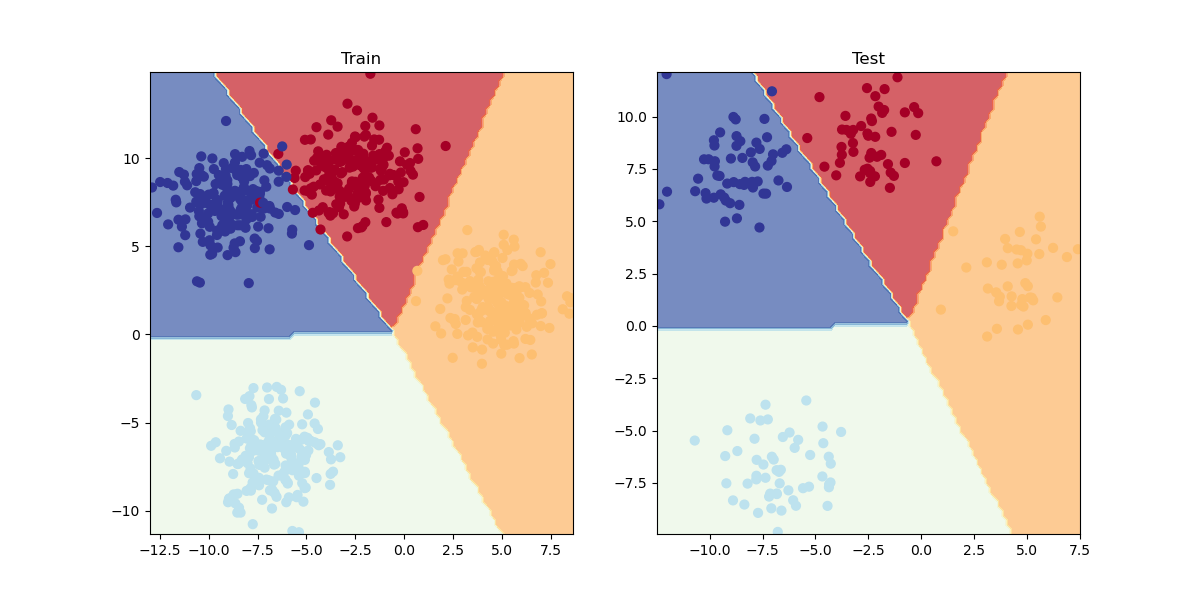
da notare che vista la distribuzioni dei "blobs" non è necessario utilizzare funzioni non lineare come la ReLU, questo perchè i dati dei blobs sono "separabili linearmente", il che significa che i dati dei blobs non si michiano in maniera non lineare come per es. nel caso di due cerchi concentrici di blobs.
Il cui output è:
Python 3.10.8 | packaged by conda-forge | (main, Nov 24 2022, 14:07:00) [MSC v.1916 64 bit (AMD64)]
Type 'copyright', 'credits' or 'license' for more information
IPython 8.7.0 -- An enhanced Interactive Python. Type '?' for help.
PyDev console: using IPython 8.7.0
Python 3.10.8 | packaged by conda-forge | (main, Nov 24 2022, 14:07:00) [MSC v.1916 64 bit (AMD64)] on win32
runfile('C:\\lavori\\formazione_py\\src\\formazione\\DanielBourkePytorch\\03_multiclass_classification.py', wdir='C:\\lavori\\formazione_py\\src\\formazione\\DanielBourkePytorch')
tensor([[-8.4134,  6.9352],
        [-5.7665, -6.4312],
        [-6.0421, -6.7661],
        [ 3.9508,  0.6984],
        [ 4.2505, -0.2815]]) tensor([3, 2, 2, 1, 1])
Epoch: 0 | Loss: 1.42610, Acc: 24.12% | Test Loss: 1.14118, Test Acc: 55.00%
Epoch: 10 | Loss: 0.69430, Acc: 71.25% | Test Loss: 0.59211, Test Acc: 78.00%
Epoch: 20 | Loss: 0.54481, Acc: 72.88% | Test Loss: 0.45338, Test Acc: 79.50%
Epoch: 30 | Loss: 0.46979, Acc: 73.12% | Test Loss: 0.38420, Test Acc: 79.00%
Epoch: 40 | Loss: 0.43818, Acc: 73.12% | Test Loss: 0.35307, Test Acc: 79.00%
Epoch: 50 | Loss: 0.42259, Acc: 77.38% | Test Loss: 0.33220, Test Acc: 93.00%
Epoch: 60 | Loss: 0.12337, Acc: 99.00% | Test Loss: 0.09245, Test Acc: 99.50%
Epoch: 70 | Loss: 0.06762, Acc: 99.00% | Test Loss: 0.05245, Test Acc: 99.50%
Epoch: 80 | Loss: 0.05137, Acc: 99.00% | Test Loss: 0.03963, Test Acc: 99.50%
Epoch: 90 | Loss: 0.04380, Acc: 99.12% | Test Loss: 0.03331, Test Acc: 99.50%
Backend MacOSX is interactive backend. Turning interactive mode on.