Workflow + regressione lineare
Introduzione
Iniziamo a trattare la regressione che nella pratica risulta essere la predizione di un numero a differenza per es. della classificazione che tratta la previsione di un "tipo", es. cats vs dogs.
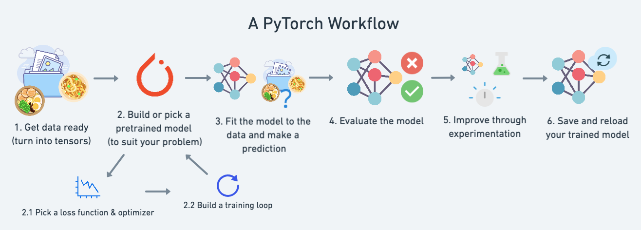
In questa lezione vedremo un tipo "torch workflow" in salsa "vanilla", basico ma utile per comprendere gli step logici. Di seguito una rappresentazione grafica del flow:
| **Topic** | **Contents** |
|---|---|
| 1 Getting data ready** | Data can be almost anything but to get started we're going to create a simple straight line |
| 2 Building a model** | Here we'll create a model to learn patterns in the data, we'll also choose a **loss function**, **optimizer** and build a **training loop**. |
| 3 Fitting the model to data (training)** | We've got data and a model, now let's let the model (try to) find patterns in the (**training**) data. |
| 4 Making predictions and evaluating a model (inference)** | Our model's found patterns in the data, let's compare its findings to the actual (**testing**) data. |
| 5 Saving and loading a model** | You may want to use your model elsewhere, or come back to it later, here we'll cover that. |
| 6 Putting it all together** | Let's take all of the above and combine it. |
Torch.NN
Per costruire una rete neurale possiamo iniziare da torch.NN dove per .nn si vuole indicare Neural Network
Preparazione dei dati
La fase iniziare e una delle più importanti nel ML è la preparazione dei dati, es:
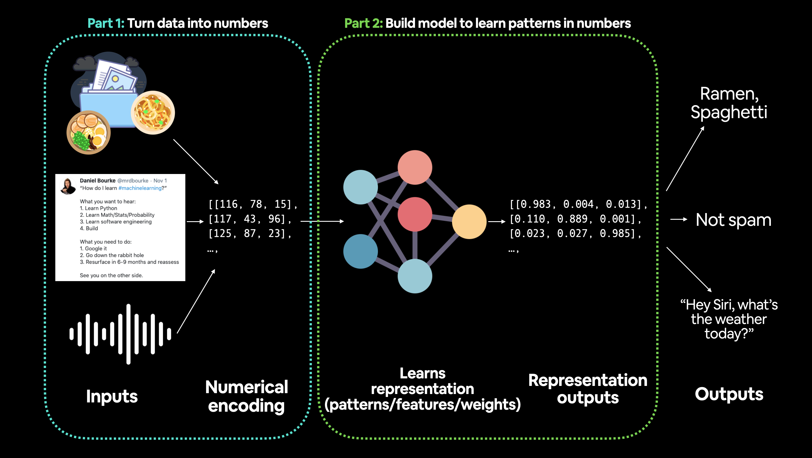
Gli step principali nella preparazione dei dati sono:
- trasforare i dati in una rappresentazione numerica
- costruire un modello che impari o scopra dei "pattern" nella rappresentazione numerica definita per il modello che vogliamo analizzare
Inziamo utilizzando la classica regressione lineare utilizzando la formula base y = wx + b, dove b sono i bias (detta intercetta) e w i pesi o coefficiente angolare. Per un approfondimento sulla regressione lineare vedi corso https://cms.marcocucchi.it/books/machine-learing/page/regressione-lineare
Ma andiamo al codice
# settiamo in parametri dell'equazione
weight = 0.7
bias = 0.3

# creiamo i dati
start = 0
end = 1
step = 0.02
# agigungo una dimensione extra tramite l'unsqueeze
X = torch.arange(start, end, step).unsqueeze(dim=1)
y = weight * X + bias

X.shape, X[:10], y[:10]

>(torch.Size([50, 1]),
(tensor([[0.0000],
         [0.0200],
         [0.0400],
         [0.0600],
         [0.0800],
         [0.1000],
         [0.1200],
         [0.1400],
         [0.1600],
         [0.1800]]),
 tensor([[0.3000],
         [0.3140],
         [0.3280],
         [0.3420],
         [0.3560],
         [0.3700],
         [0.3840],
         [0.3980],
         [0.4120],
         [0.4260]]))
Nell'esempio sopra riportato andremo a creare i dati relativi ad una semplice equazione lineare che verranno inviati alla rete neurale per identificare il pattern che più si avvicina all'equazione Y= vw + b che li ha originati
Training, Validation e Test sets
Uno dei concetti più importanti nel ML è la suddivisione dei dati in tre grupi:
| Split | Purpose | Amount of total data | How often is it used? |
|---|---|---|---|
| **Training set** | sono i dati sui quali il Pytoch si "allena" per trovare il modello | ~60-80% | Always |
| **Validation set** | Non sempre utilizzato, nella pratica serve per effettuare una validazione interna del training. Da notare che questi non vengono utilizzati nella fase di training, servono solo per una validazione del modello in fase di training. | ~10-20% | Often but not always |
| **Testing set** | Validazione finare del modello. | ~10-20% | Always |
Come splittare i dati i dati in training e testing:
# Create train/test split
train_split = int(0.8 * len(X)) # 80% of data used for training set, 20% for testing
X_train, y_train = X[:train_split], y[:train_split]
X_test, y_test = X[train_split:], y[train_split:]

len(X_train), len(y_train), len(X_test), len(y_test)
in questo modo dividiamo i dati dove l'80% sono dedicati al training e il restante 20% per la fase di test
Visualizziamo ora i dati:
def plot_predictions(train_data=X_train,
                     train_labels=y_train,
                     test_data=X_test,
                     test_labels=y_test,
                     predictions=None):
  """
  Plots training data, test data and compares predictions.
  """
  plt.figure(figsize=(10, 7))

  # Plot training data in blue
  plt.scatter(train_data, train_labels, c="b", s=4, label="Training data")

  # Plot test data in green
  plt.scatter(test_data, test_labels, c="g", s=4, label="Testing data")

  if predictions is not None:
    # Plot the predictions in red (predictions were made on the test data)
    plt.scatter(test_data, predictions, c="r", s=4, label="Predictions")

  # Show the legend
  plt.legend(prop={"size": 14});

plot_predictions();
e l'output risulta:
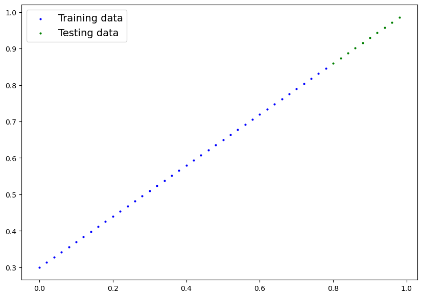
in blu i dati di traing, mentre in verde quelli di test.
Ora creiamo il modello:
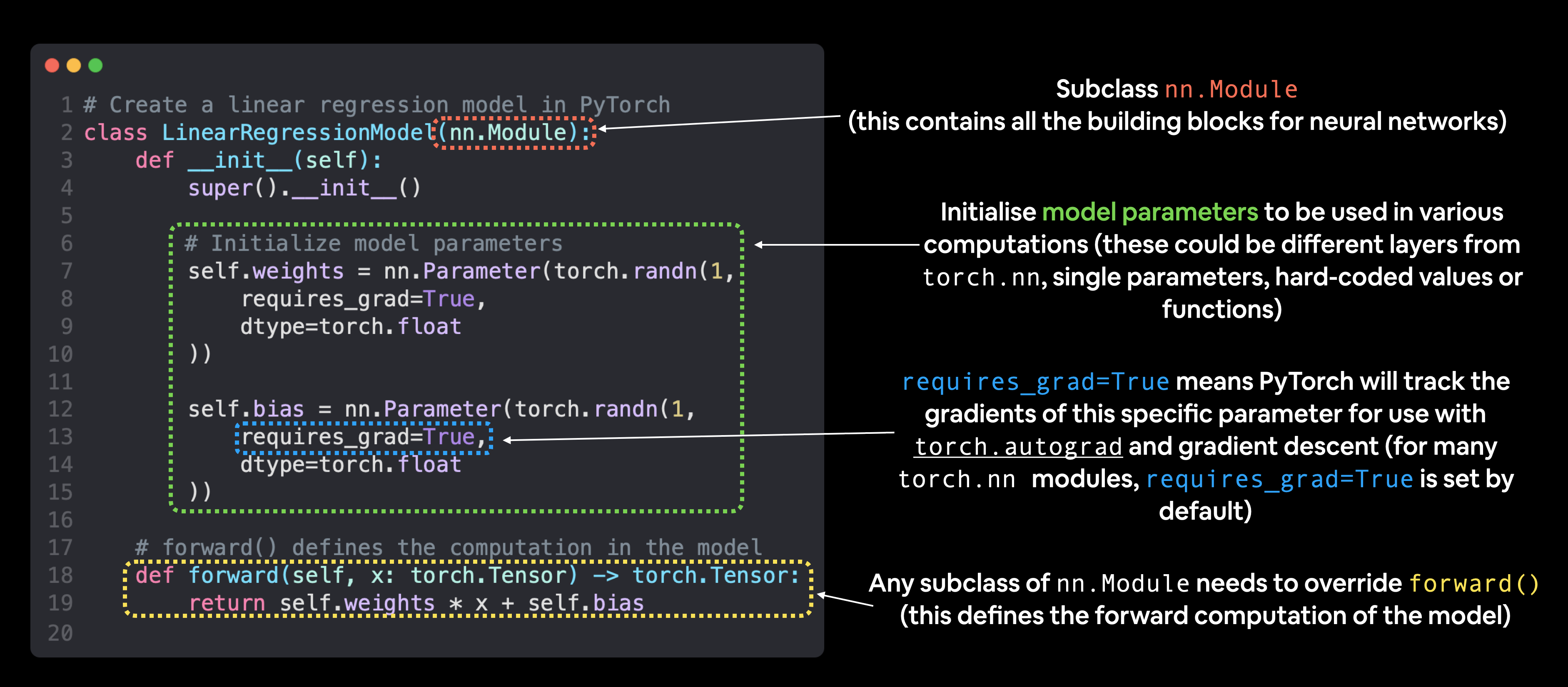
# Creiamo un classe di regressione lineare che eredita da nn.Module
class LinearRegressionModel(nn.Module):

    # inizializzazione delle rete neurale
    def __init__(self):
        super().__init__()

        # normalmente le w e b sono più complesso di questo caso...
        # il nome di questo tipo di variabili è arbitrario
        self.weights = nn.Parameter(torch.randn(1, # generiamo un (1) tensore con un valore randomico
                                              dtype=torch.float), # <- PyTorch preferisce utilizzare float32 by default
                                             requires_grad=True) # pytoch aggiornerà il parametro tramite il backpropagation e discesa del gradiente

        # il nome di questo tipo di variabili è arbitrario
        self.bias = nn.Parameter(torch.randn(1, # generiamo un (1) tensore con un valore randomico
                                            dtype=torch.float), # <- PyTorch preferisce utilizzare float32 by default
                                            requires_grad=True)  # pytoch aggiornerà il parametro tramite il backpropagation e discesa del gradiente


    # propagazione di tipo "forward"
    def forward(self, x: torch.Tensor) -> torch.Tensor: # <- "x"  input data (training/testing features)
        return self.weights * x + self.bias # <- questa è la formula della regressione lineare (y = m*x + b)
La classe torch.NN è la base per la creazione dei "grafi di neuroni", questa classe effettua due macro tipologie di operazioni, ovvero:
- la discesa del gradiente
- la Backpropagation
tenendo traccia della variazione dei pesi e dei bias.
Il metodo "torch.randn" può generare un tensore il cui shape è passato in input es.
torch.randn(2, 3)
PyTorch model building essentials
Le componenti princiali (più o meno) per creare una rete neurale in Pytorch sono:
torch.nn, torch.optim, torch.utils.data.Dataset and torch.utils.data.DataLoader. For now, we'll focus on the first two and get to the other two later (though you may be able to guess what they do).
| PyTorch module | What does it do? |
|---|---|
| torch.nn | Contains all of the building blocks for computational graphs (essentially a series of computations executed in a particular way). |
| torch.nn.Parameter | Stores tensors that can be used with `nn.Module`. If `requires_grad=True` gradients (used for updating model parameters via [**gradient descent**](https://ml-cheatsheet.readthedocs.io/en/latest/gradient_descent.html)) are calculated automatically, this is often referred to as "autograd". |
| torch.nn.Module | The base class for all neural network modules, all the building blocks for neural networks are subclasses. If you're building a neural network in PyTorch, your models should subclass `nn.Module`. Requires a `forward()` method be implemented. |
| torch.optim | Contains various optimization algorithms (these tell the model parameters stored in `nn.Parameter` how to best change to improve gradient descent and in turn reduce the loss). |
| def forward() | All `nn.Module` subclasses require a `forward()` method, this defines the computation that will take place on the data passed to the particular `nn.Module` (e.g. the linear regression formula above).
Questa classe in genere va sempre implementata |
If the above sounds complex, think of like this, almost everything in a PyTorch neural network comes from torch.nn,
nn.Modulecontains the larger building blocks (layers)nn.Parametercontains the smaller parameters like weights and biases (put these together to makenn.Module(s))forward()tells the larger blocks how to make calculations on inputs (tensors full of data) withinnn.Module(s)torch.optimcontains optimization methods on how to improve the parameters withinnn.Parameterto better represent input data
Visualizziamo i valori w e b prima dell'elaboraizone:
# Set manual seed since nn.Parameter are randomly initialzied
torch.manual_seed(42)

# Create an instance of the model (this is a subclass of nn.Module that contains nn.Parameter(s))
model_0 = LinearRegressionModel()

# Check the nn.Parameter(s) within the nn.Module subclass we created
list(model_0.parameters())

>[Parameter containing:
 tensor([0.3367], requires_grad=True),

# vediamo la lista dei parametri
model_0.state_dict()
>OrderedDict([('weights', tensor([0.3367])), ('bias', tensor([0.1288]))])
proviamo a fare delle predizioni senza aver fatto il training giusto per vedere come si comporta il modello.
Per fare delle predizioni si utilizza il medoto .inference_mode():
# Make predictions with model
# con torch.inference_mode() facciamo in modo non si salvi i parametri che normalmente vengono
# utilizzati nella fase di training, cosa inutile durante la predizione in quanto il training
# dovrebbe essere già stato effettuato. In soldoni migliori performace durante la fare predittiva
with torch.inference_mode():
    y_preds = model_0(X_test)

# Check the predictions
print(f"Number of testing samples: {len(X_test)}")
print(f"Number of predictions made: {len(y_preds)}")
print(f"Predicted values:\n{y_preds}")

Number of testing samples: 10
Number of predictions made: 10
Predicted values:
tensor([[0.3982],
        [0.4049],
        [0.4116],
        [0.4184],
        [0.4251],
        [0.4318],
        [0.4386],
        [0.4453],
        [0.4520],
        [0.4588]])

# proviamo a visualizzare i valori della previsione
plot_predictions(predictions=y_preds)
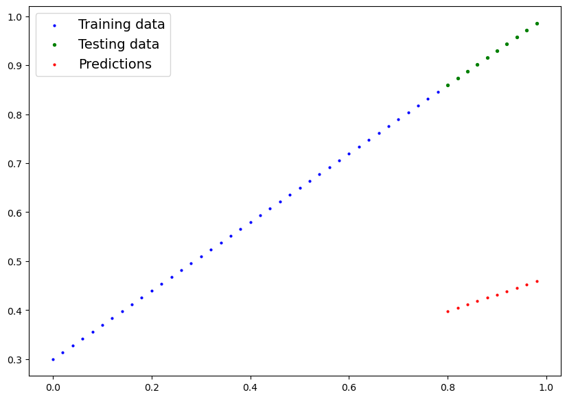
e come si bene notare i valori predetti (rosso) "poco ci azzeccano" con i valori originali... quindi le predizioni sono praticamente random.
Training
Loss function
Prima di trattare il training per se vediamo di capire come misura quanto il modello si avvicina ai valori attesi o ideali, per effettuare questo controllo viene utilizzata la "loss function" o "cost function". (vedo https://pytorch.org/docs/stable/nn.html#loss-functions)
Nella pratica uno dei metodi più basici è misurare la distanza tra gli attesi e i predetti.
Optimizer
L'optimizer serve per ottimizzare i valori predetti in modo che si avvicinino sempre di più ai valori ideali, quindi per migliorare la loss function. (i cui delta vengono ritornati dalla "loss function", in modo che la loss function stessa indichi un miglioramento della predizione)
Nello specifico per pytorch servirà un training loop e un test loop.
Creare una loss function e un optimizer
| Function | What does it do? | Where does it live in PyTorch? | Common values |
|---|---|---|---|
| **Loss function** | Measures how wrong your models predictions (e.g. `y_preds`) are compared to the truth labels (e.g. `y_test`). Lower the better.
vedi tabella delle loss functions: |
PyTorch has plenty of built-in loss functions in [`torch.nn`](https://pytorch.org/docs/stable/nn.html#loss-functions). | Mean absolute error (MAE) for regression problems ([`torch.nn.L1Loss()`](https://pytorch.org/docs/stable/generated/torch.nn.L1Loss.html)). Binary cross entropy for binary classification problems ([`torch.nn.BCELoss()`](https://pytorch.org/docs/stable/generated/torch.nn.BCELoss.html)). |
| **Optimizer** | Tells your model how to update its internal parameters to best lower the loss.
vedi lista degli optimizers |
You can find various optimization function implementations in [`torch.optim`](https://pytorch.org/docs/stable/optim.html). | Stochastic gradient descent ([`torch.optim.SGD()`](https://pytorch.org/docs/stable/generated/torch.optim.SGD.html#torch.optim.SGD)). Adam optimizer ([`torch.optim.Adam()`](https://pytorch.org/docs/stable/generated/torch.optim.Adam.html#torch.optim.Adam)). |
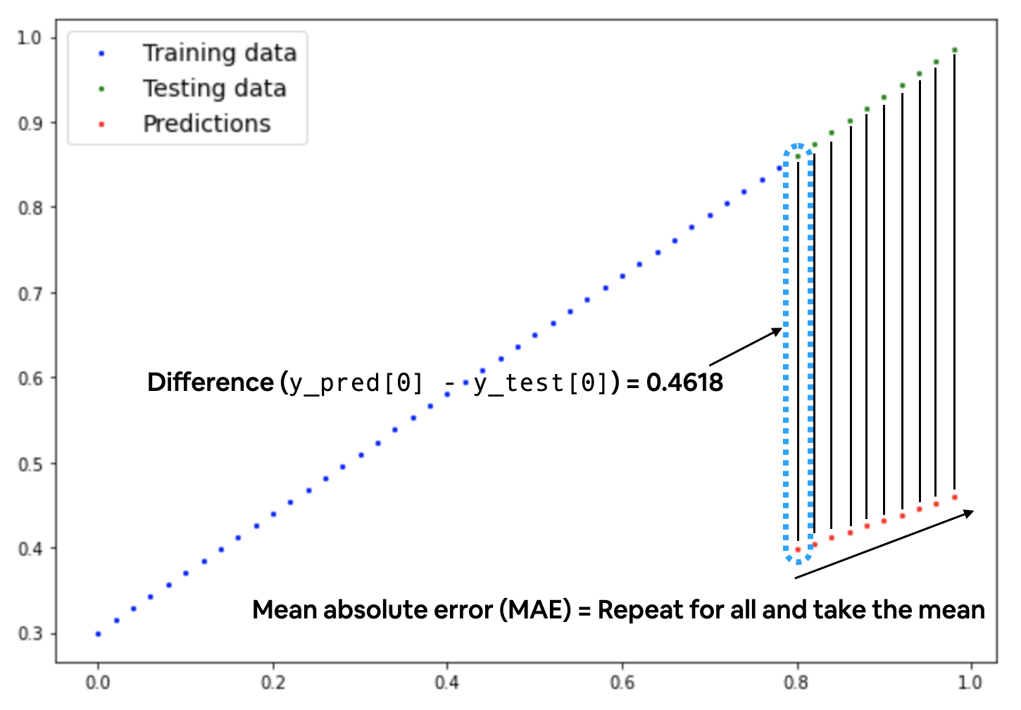
Esistono varie famiglie di "loss function" a seconda del tipo di elaborazione, per la predizioni di valori numerici è possibile utilizzare la Mean absolute error (MAE, in PyTorch: torch.nn.L1Loss) che miura la differenze in valori assoluti tra due punti che nel nostro caso sono le "prediction" e le "label" (che sono i valori attesi) per poi calcolarne il valore medio.
Di seguito una rappresentazione grafica dello MAE, dove si evidenzia il calcolo medio della differenza in valore assoulto tra valori attesi e valori predetti.
quindi:
# creiamo una loss function
loss_fn = nn.L1Loss() # MAE

# creiamo un optimizer, scegliamo il classico Stocastic Gradient Descent
optimizer = torch.optim.SGD(params=model_0.parameters(), # passiamo i parametri da ottimizzare (in questo caso "w" e "b"
                            lr=0.01) # settiamo il passo per il calcolo del gradiente, più piccolo = più tempo
di seguito gli step logici della fare si training:
PyTorch training loop
For the training loop, we'll build the following steps:
| Number | Step name | What does it do? | Code example |
|---|---|---|---|
| 1 | Forward pass | The model goes through all of the training data once, performing its `forward()` function calculations. | `model(x_train)` |
| 2 | Calculate the loss | The model's outputs (predictions) are compared to the ground truth and evaluated to see how wrong they are. | `loss = loss_fn(y_pred, y_train)` |
| 3 | Zero gradients | The optimizers gradients are set to zero (they are accumulated by default) so they can be recalculated for the specific training step. | `optimizer.zero_grad()` |
| 4 | Perform backpropagation on the loss | Computes the gradient of the loss with respect for every model parameter to be updated (each parameter with `requires_grad=True`). This is known as **backpropagation**, hence "backwards". | `loss.backward()` |
| 5 | Update the optimizer (**gradient descent**) | Update the parameters with `requires_grad=True` with respect to the loss gradients in order to improve them. | `optimizer.step()` |
l'algoritmo quindi si può delineare come:
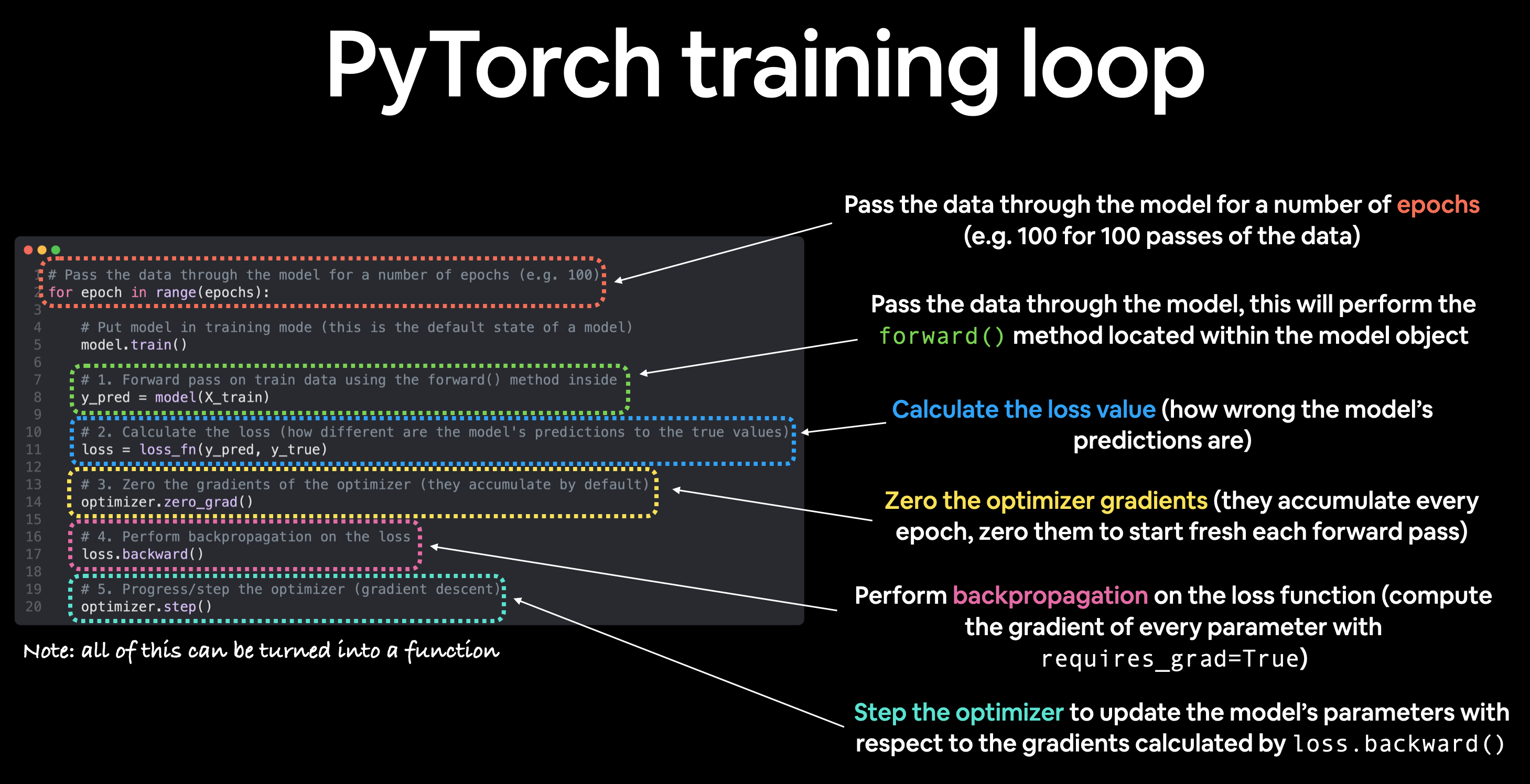
di seguito l'algoritmo:
# forzo il seed per ottenere risultati identici al
torch.manual_seed(42)

# setto le epoche, ogni epoca è un passaggio in "foward propagation" dei pesi attraverso la rete neurale
# dall'input layer all'ouout.
epochs = 100

# creo delle liste che conterranno i valori di loss per tenerne traccia durante le varie epche
train_loss_values = []
test_loss_values = []
epoch_count = []

for epoch in range(epochs):
    ### Training

    # 0. imposto la modalità in Training (da fare ad ogni epoca)
    model_0.train()

    # 1. passo i dati di training al modello il quale internamente invocherè il metoto forward() definito
    #    quanto è stata implementata la classe che estende pytorch. Ottengo i dati che andranno poi comprati
    #    dalla loss per ottenerne in valore medio assoluto.
    y_pred = model_0(X_train)
    # print(y_pred)

    # 2. calcolo la loss utilizzando la funzione definita precedentemmente.
    loss = loss_fn(y_pred, y_train)

    # 3. reinizializzo l'optimizer in quanto tende ad accumulare i valori
    optimizer.zero_grad()

    # 4. effettua la back propagation, nella pratica Pytorch tiene traccia dei valori associati alla discesa del gradiente
    #    Quindi calcola la derivata parziale per determinare il minimo della curva dei delta tra valori predetti e valori di test
    loss.backward()

    # 5. ottimizza i parametri (una sola volta) e in base al valore "lr".
    #  NB: cambia quindi i valori dei tensori per cercare di farli avvicinare ai valori ottimali
    optimizer.step()

    ### Testing

    # indico a Pytrch che la fase di training è terminata e che ora devo valutare i parametri e paragonarli con i valori attesi
    model_0.eval()

    # predico i valori in
    with torch.inference_mode():
      # 1. Forward pass on test data
      test_pred = model_0(X_test)

      # 2. Caculate loss on test data
      test_loss = loss_fn(test_pred, y_test.type(torch.float)) # predictions come in torch.float datatype, so comparisons need to be done with tensors of the same type

      # Print out what's happening
      if epoch % 10 == 0:
            epoch_count.append(epoch)
          	# i valori vengono convertiti in numpy in quanto sono dei tensori pytorch
            train_loss_values.append(loss.numpy())
            test_loss_values.append(test_loss.numpy())
            print(f"Epoch: {epoch} | MAE Train Loss: {loss} | MAE Test Loss: {test_loss} ")
e l'output sarà:
print (list(model_0.parameters()),model_0.state_dict())

Epoch: 0 | MAE Train Loss: 0.31288138031959534 | MAE Test Loss: 0.48106518387794495 delta: 0.1681838035583496
Epoch: 10 | MAE Train Loss: 0.1976713240146637 | MAE Test Loss: 0.3463551998138428 delta: 0.14868387579917908
Epoch: 20 | MAE Train Loss: 0.08908725529909134 | MAE Test Loss: 0.21729660034179688 delta: 0.12820935249328613
Epoch: 30 | MAE Train Loss: 0.053148526698350906 | MAE Test Loss: 0.14464017748832703 delta: 0.09149165451526642
Epoch: 40 | MAE Train Loss: 0.04543796554207802 | MAE Test Loss: 0.11360953003168106 delta: 0.06817156076431274
Epoch: 50 | MAE Train Loss: 0.04167863354086876 | MAE Test Loss: 0.09919948130846024 delta: 0.057520847767591476
Epoch: 60 | MAE Train Loss: 0.03818932920694351 | MAE Test Loss: 0.08886633068323135 delta: 0.05067700147628784
Epoch: 70 | MAE Train Loss: 0.03476089984178543 | MAE Test Loss: 0.0805937647819519 delta: 0.04583286494016647
Epoch: 80 | MAE Train Loss: 0.03132382780313492 | MAE Test Loss: 0.07232122868299484 delta: 0.040997400879859924
Epoch: 90 | MAE Train Loss: 0.02788739837706089 | MAE Test Loss: 0.06473556160926819 delta: 0.03684816509485245
Epoch: 100 | MAE Train Loss: 0.024458957836031914 | MAE Test Loss: 0.05646304413676262 delta: 0.032004088163375854
Epoch: 110 | MAE Train Loss: 0.021020207554101944 | MAE Test Loss: 0.04819049686193466 delta: 0.027170289307832718
Epoch: 120 | MAE Train Loss: 0.01758546568453312 | MAE Test Loss: 0.04060482233762741 delta: 0.02301935665309429
Epoch: 130 | MAE Train Loss: 0.014155393466353416 | MAE Test Loss: 0.03233227878808975 delta: 0.018176885321736336
Epoch: 140 | MAE Train Loss: 0.010716589167714119 | MAE Test Loss: 0.024059748277068138 delta: 0.01334315910935402
Epoch: 150 | MAE Train Loss: 0.0072835334576666355 | MAE Test Loss: 0.016474086791276932 delta: 0.009190553799271584
Epoch: 160 | MAE Train Loss: 0.0038517764769494534 | MAE Test Loss: 0.008201557211577892 delta: 0.004349780734628439
Epoch: 170 | MAE Train Loss: 0.008932482451200485 | MAE Test Loss: 0.005023092031478882 delta: -0.003909390419721603
Epoch: 180 | MAE Train Loss: 0.008932482451200485 | MAE Test Loss: 0.005023092031478882 delta: -0.003909390419721603
[Parameter containing:
tensor([0.6990], requires_grad=True), Parameter containing:
tensor([0.3093], requires_grad=True)] OrderedDict([('weights', tensor([0.6990])), ('bias', tensor([0.3093]))])
Mostriamo il grafico dei loss sul training e sui dati di testing
# Plot the loss curves
plt.plot(epoch_count, train_loss_values, label="Train loss")
plt.plot(epoch_count, test_loss_values, label="Test loss")
plt.title("Training and test loss curves")
plt.ylabel("Loss")
plt.xlabel("Epochs")
plt.legend();
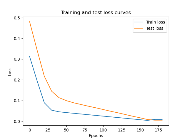
e vediamo il grafico dei valori predetti vs i valori utilizzati per il traing
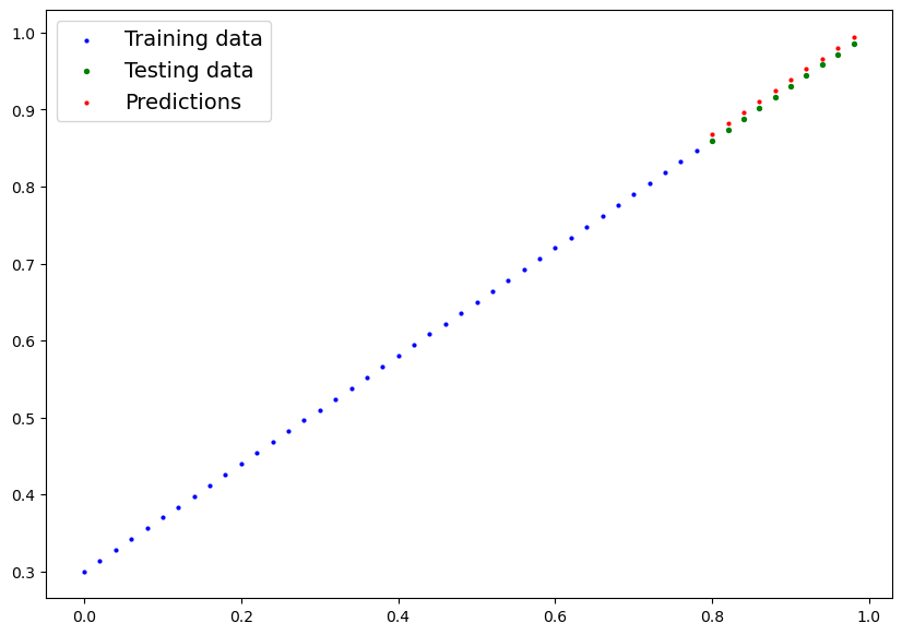
si può notare che dopo 180 epoche di training il modello riesce a predirre valori molto simili a quelli utilizzati per il training.
Salvare e caricare i parametri del modello
Dopo avere trovato i valori che meglio rappresentano il modello che vogliamo riprodurre vogliamo salvare i valori della rete neurale in modo da poterli ricaricare in un secondo momento senza dover riallenare la rete. Pytorch mette a disposizioni i metodo save e load per salvare su file system i parametri.
| PyTorch method | What does it do? |
|---|---|
| torch.save | Saves a serialzed object to disk using Python's [`pickle`](https://docs.python.org/3/library/pickle.html) utility. Models, tensors and various other Python objects like dictionaries can be saved using `torch.save`. |
| torch.load) | Uses `pickle`'s unpickling features to deserialize and load pickled Python object files (like models, tensors or dictionaries) into memory. You can also set which device to load the object to (CPU, GPU etc). |
| torch.nn.Module.load_state_dict | Loads a model's parameter dictionary (`model.state_dict()`) using a saved `state_dict()` object |
from pathlib import Path

# 1. Create models directory
MODEL_PATH = Path("C:/Users/userxx/Desktop")

MODEL_PATH.mkdir(parents=True, exist_ok=True)

# 2. Create model save path
MODEL_NAME = "01_pytorch_workflow_model_0.pth"
MODEL_SAVE_PATH = MODEL_PATH / MODEL_NAME

# 3. Save the model state dict
print(f"Saving model to: {MODEL_SAVE_PATH}")
torch.save(obj=model_0.state_dict(), # only saving the state_dict() only saves the models learned parameters
           f=MODEL_SAVE_PATH)
verrà quindi creato un file con i bias e i weights, per caricare il modello invce:
# Instantiate a new instance of our model (this will be instantiated with random weights)
loaded_model_0 = LinearRegressionModel()

# Load the state_dict of our saved model (this will update the new instance of our model with trained weights)
loaded_model_0.load_state_dict(torch.load(f=MODEL_SAVE_PATH))
e provare il modello caricato:
# 1. Put the loaded model into evaluation mode
loaded_model_0.eval()

# 2. Use the inference mode context manager to make predictions
with torch.inference_mode():
    loaded_model_preds = loaded_model_0(X_test) # perform a forward pass on the test data with the loaded model
Evoluzione del modello/uso della GPU
Creiamo ora un modello in grado di gestire un numero significativamente maggiore di layers e nuroni configurandoli più facilmente:
# Subclass nn.Module to make our model
class LinearRegressionModelV2(nn.Module):
    def __init__(self):
        super().__init__()

        # utilizziamo un layer di quelli predefiniti da pytorch
        # questa volta definiamo una semplice rete neurale fatta di un input layer e un output layer
        # il modello libeare si basa sulla classica formula y = w*x + b
        self.linear_layer = nn.Linear(in_features=1,
                                      out_features=1)

    # Definiamo la "forward computation" dove i valori i input "scorrono" attraverso
    # la rete neurale defininta nel costruttore della classe
    def forward(self, x: torch.Tensor) -> torch.Tensor:
        return self.linear_layer(x)

# setto il seed per facilitare il check dei paramertri
torch.manual_seed(42)
model_1 = LinearRegressionModelV2()

print( model_1)
>LinearRegressionModelV2( (linear_layer): Linear(in_features=1, out_features=1, bias=True) )

print( model_1.state_dict())
>OrderedDict([('linear_layer.weight', tensor([[0.7645]])), ('linear_layer.bias', tensor([0.8300]))])
vediamo di forzare l'uso della GPU, se presente:
# Setup device agnostic code
device = "cuda" if torch.cuda.is_available() else "cpu"
print(f"Using device: {device}")
> Using device: cuda

# Check model device
next(model_1.parameters()).device
>device(type='cpu')
si evince che di default viene la utilizzata la CPU, il nostro intente invece è utilizzare la GPU se presente e creare un sistema "agnostico" in grado di sfruttare le risorse al meglio, per cui settiamo il decice migliore:
# Set model to GPU if it's availalble, otherwise it'll default to CPU
model_1.to(device) # the device variable was set above to be "cuda" if available or "cpu" if not
next(model_1.parameters()).device

# ora utilizza la GPU
>device(type='cuda', index=0)
ripetiamo il training con il nuovo modello:
# Create loss function
loss_fn = nn.L1Loss()

# Create optimizer
optimizer = torch.optim.SGD(params=model_1.parameters(), # optimize newly created model's parameters
                            lr=0.01)

torch.manual_seed(42)

# Set the number of epochs
epochs = 1000

# !!!!!!!!!!!!!
# Put data on the available device
# Without this, error will happen (not all model/data on device)
# !!!!!!!!!!!!!
X_train = X_train.to(device)
X_test = X_test.to(device)
y_train = y_train.to(device)
y_test = y_test.to(device)

for epoch in range(epochs):
    ### Training
    model_1.train() # train mode is on by default after construction

    # 1. Forward pass
    y_pred = model_1(X_train)

    # 2. Calculate loss
    loss = loss_fn(y_pred, y_train)

    # 3. Zero grad optimizer
    optimizer.zero_grad()

    # 4. Loss backward
    loss.backward()

    # 5. Step the optimizer
    optimizer.step()

    ### Testing
    model_1.eval() # put the model in evaluation mode for testing (inference)
    # 1. Forward pass
    with torch.inference_mode():
        test_pred = model_1(X_test)

        # 2. Calculate the loss
        test_loss = loss_fn(test_pred, y_test)

    if epoch % 100 == 0:
        print(f"Epoch: {epoch} | Train loss: {loss} | Test loss: {test_loss}")
e l'output:
# Find our model's learned parameters
from pprint import pprint # pprint = pretty print, see: https://docs.python.org/3/library/pprint.html
print("The model learned the following values for weights and bias:")
pprint(model_1.state_dict())
print("\nAnd the original values for weights and bias are:")
print(f"weights: {weight}, bias: {bias}")

The model learned the following values for weights and bias:
OrderedDict([('linear_layer.weight', tensor([[0.6968]], device='cuda:0')),
             ('linear_layer.bias', tensor([0.3025], device='cuda:0'))])

And the original values for weights and bias are:
weights: 0.7, bias: 0.3
Fare delle previsioni
# Turn model into evaluation mode
model_1.eval()

# Make predictions on the test data
with torch.inference_mode():
    y_preds = model_1(X_test)

print(y_preds)
tensor([[0.8600],
        [0.8739],
        [0.8878],
        [0.9018],
        [0.9157],
        [0.9296],
        [0.9436],
        [0.9575],
        [0.9714],
        [0.9854]], device='cuda:0')
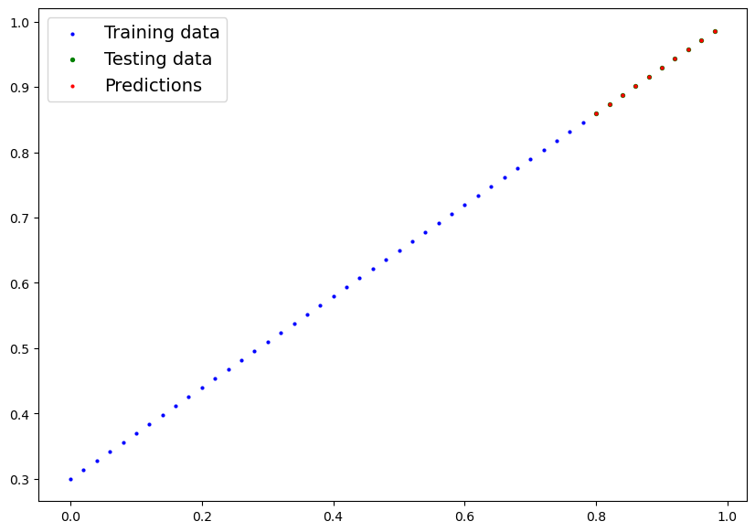
Facciamo il plot ma attenzione che i tensori sono nella GPU mentre la funzione di plot lavora con la CPU (numpy), bisognerà quindi trasferire i valori in numpy primna di plottarli.
plot_predictions(predictions=y_preds) # -> non funziona in quanto i dati sono nella GPU
>TypeError: can't convert cuda:0 device type tensor to numpy. Use Tensor.cpu() to copy the tensor to host memory first.

# Put data on the CPU and plot it
plot_predictions(predictions=y_preds.cpu())
Salvare il modello
from pathlib import Path

# 1. Create models directory
MODEL_PATH = Path("path alla directoty dei modelli")
MODEL_PATH.mkdir(parents=True, exist_ok=True)

# 2. Create model save path
MODEL_NAME = "01_pytorch_workflow_model_1.pth"
MODEL_SAVE_PATH = MODEL_PATH / MODEL_NAME

# 3. Save the model state dict
print(f"Saving model to: {MODEL_SAVE_PATH}")
torch.save(obj=model_1.state_dict(), # only saving the state_dict() only saves the models learned parameters
           f=MODEL_SAVE_PATH)
Caricare il modello
# Instantiate a fresh instance of LinearRegressionModelV2
loaded_model_1 = LinearRegressionModelV2()

# Load model state dict
loaded_model_1.load_state_dict(torch.load(MODEL_SAVE_PATH))

# Put model to target device (if your data is on GPU, model will have to be on GPU to make predictions)
loaded_model_1.to(device)

print(f"Loaded model:\n{loaded_model_1}")
print(f"Model on device:\n{next(loaded_model_1.parameters()).device}")
testare il modello caricato
# Evaluate loaded model
loaded_model_1.eval()
with torch.inference_mode():
    loaded_model_1_preds = loaded_model_1(X_test)
y_preds == loaded_model_1_preds

>tensor([[True],
        [True],
        [True],
        [True],
        [True],
        [True],
        [True],
        [True],
        [True],
        [True]], device='cuda:0')