Classificazione

Introduzione

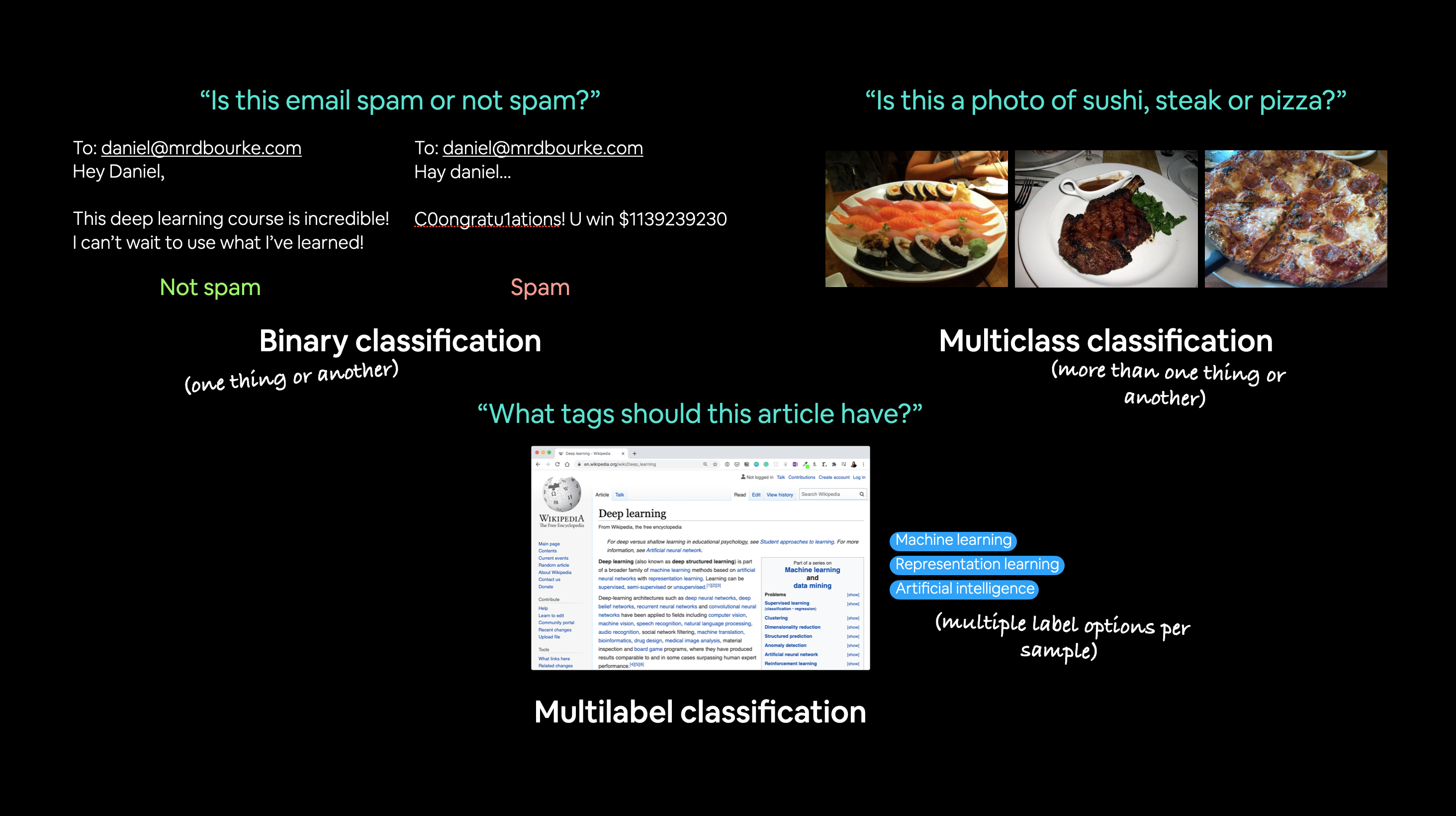
In questa lezione andremo a vedere la classificazione in base a delle tipolgie di dati, differisce quindi dalla regressione che si basa sulla predizione di un valore numero.

La classificazione può essere "binaria" es. cats vs dogs, oppure multiclass classification se abbiamo più di due tipologie da classificare.

Di seguito alcuni esempi di classificazione:

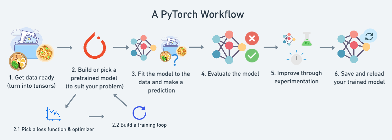
Cosa andreamo a trattare nel coso:

Topic	Contents
0. Architecture of a classification neural network	Neural networks can come in almost any shape or size, but they typically follow a similar floor plan.
1. Getting binary classification data ready	Data can be almost anything but to get started we're going to create a simple binary classification dataset.
2. Building a PyTorch classification model	Here we'll create a model to learn patterns in the data, we'll also choose a loss function, optimizer and build a training loop specific to classification.
3. Fitting the model to data (training)	We've got data and a model, now let's let the model (try to) find patterns in the (training) data.
4. Making predictions and evaluating a model (inference)	Our model's found patterns in the data, let's compare its findings to the actual (testing) data.
5. Improving a model (from a model perspective)	We've trained an evaluated a model but it's not working, let's try a few things to improve it.
6. Non-linearity	So far our model has only had the ability to model straight lines, what about non-linear (non-straight) lines?
7. Replicating non-linear functions	We used non-linear functions to help model non-linear data, but what do these look like?
8. Putting it all together with multi-class classification	Let's put everything we've done so far for binary classification together with a multi-class classification problem.

Partiamo con un esempio di classificazione basato su due serie di cerchi che si annidano tra di loro. Utilizziamo sklearn per ottenere questo set di dati:

from sklearn.datasets import make_circles

Make 1000 samples

n_samples = 1000

X, y = make_circles(n_samples,
					noise=0.03, # a little bit of noise to the dots                    
                    random_state=42) # keep random state so we get the same values

Create circles

proviamo a vedere cosa contengono le X e le y.

print(f"First 5 X features:\n{X[:5]}")
print(f"\nFirst 5 y labels:\n{y[:5]}")

First 5 X features: [[ 0.75424625 0.23148074] [-0.75615888 0.15325888] [-0.81539193 0.17328203] [-0.39373073 0.69288277] [ 0.44220765 -0.89672343]]

First 5 y labels:[1 1 1 1 0]

quindi le X contengono delle coordinate metre le y si suddividono in valori zero e uno. Quindi siamo di fronte ad una classificazione binaria, ma vediamola graficamente:


import matplotlib.pyplot as plt
plt.scatter(x=X[:, 0],
            y=X[:, 1],
            c=y,
            cmap=plt.cm.RdYlBu);

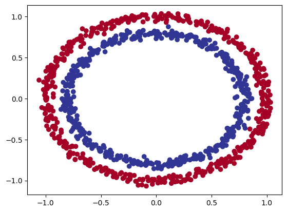
Quindi riassimento le X contengo le coordinate del cerchio, mentre le y il colore. Dalla figura si vede che i cerchi sono suffidivisi in due macrogruppi posizionati uno all'interno dell'altro.

Vediamo le shape:

# Check the shapes of our features and labels
X.shape, y.shape

((1000, 2), (1000,))

X ha una shape di due, mentre le y non ha uno shape in quanto è uno scalare di un valore.

Ora converiamo da numpy a tensori

# Turn data into tensors
# Otherwise this causes issues with computations later on
import torch
X = torch.from_numpy(X).type(torch.float)
y = torch.from_numpy(y).type(torch.float)

View the first five samples

print (X[:5], y[:5])

(tensor([[ 0.7542, 0.2315],[-0.7562, 0.1533],[-0.8154, 0.1733],[-0.3937, 0.6929],[ 0.4422, -0.8967]]),tensor([1., 1., 1., 1., 0.]))

lo converiamo in float32 (float) perchè numpy è in float64

splittiamo i dati in training e test

# Split data into train and test sets
from sklearn.model_selection import train_test_split

X_train, X_test, y_train, y_test = train_test_split(X, y, test_size=0.2, random_state=42) # make the random split

La funziona "train_test_split" splitta le featurues e le label per noi. :)

Bene, ora costruiamo il modello:

# Standard PyTorch imports
import torch
from torch import nn

# Make device agnostic code
device = "cuda" if torch.cuda.is_available() else "cpu" device

Construct a model class that subclasses nn.Module

class CircleModelV0(nn.Module): 
  def init(self): 
    super().init() 
    	# 2. Create 2 nn.Linear layers capable of handling X and y input and output shapes 
    	self.layer_1 = nn.Linear(in_features=2, out_features=5) 
        
        # takes in 2 features (X), produces 5 features 
        self.layer_2 = nn.Linear(in_features=5, out_features=1) # takes in 5 features, produces 1 feature (y)

	# 3. Define a forward method containing the forward pass computation
	def forward(self, x):
    	# Return the output of layer_2, a single feature, the same shape as y
    	return self.layer_2(self.layer_1(x)) # computation goes through layer_1 first then the output of layer_1 goes through layer_2

Create an instance of the model and send it to target device

model_0 = CircleModelV0().to(device)model_0

NB: una regola per settare il numero di feautres in input è fallo coincidere con le features del dataset. Idem per le features di output.

esiste inoltre un altro modo per rappresentare il modello in stile "Tensorflow", es:

# costruisco il modello
model_0 = nn.Sequential(
    nn.Linear(in_features=2, out_features=6),
    nn.Linear(in_features=6, out_features=2),
    nn.Linear(in_features=2, out_features=1)
).to(device)

model_0

Questo tipo di definizione del modello è "limitato" dal fatto che è sequenziale e quindi meno flessibile rispetto a reti più articolate.

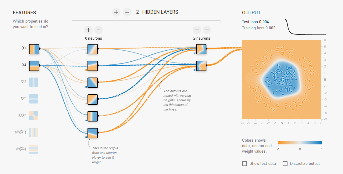
Il modello può essere rappresentato graficamente come sotto riportato:

ora, prima di fare il training del modello proviamo a passare i dati di test per vedere che output viene generato. (ovviamente essendo un modello non "allenato" saranno dati casuali)

# Make predictions with the model
with torch.inference_mode():
	untrained_preds = model_0(X_test.to(device))
	print(f"Length of predictions: {len(untrained_preds)}, Shape: {untrained_preds.shape}")
	print(f"Length of test samples: {len(y_test)}, Shape: {y_test.shape}")
	print(f"\nFirst 10 predictions:\n{untrained_preds[:10]}")
	print(f"\nFirst 10 test labels:\n{y_test[:10]}")

Length of predictions: 200, Shape: torch.Size([200, 1]) Length of test samples: 200, Shape: torch.Size([200])

First 10 predictions: tensor([[-0.7534], [-0.6841], [-0.7949], [-0.7423], [-0.5721], [-0.5315], [-0.5128], [-0.4765], [-0.8042], [-0.6770]], device='cuda:0', grad_fn=<SliceBackward0>)

First 10 test labels:tensor([1., 0., 1., 0., 1., 1., 0., 0., 1., 0.])

Possiamo notare che che l'output non è zero oppure uno come invce sono le labels... come mai? lo vedremo più avanti...

Prima di fare il training settiamo la "loss function" e "l'optimizer".

Setup loss function and optimizer

La domanda che ci si pone di sempre quale loss function e optimizer utilzzare?

Per la classfificazione in genere si utilizza la binary cross entropy, vedi tabella esempio sotto ripotata:

Loss function/Optimizer	Problem type	PyTorch Code
Stochastic Gradient Descent (SGD) optimizer	Classification, regression, many others.	[`torch.optim.SGD()`](https://pytorch.org/docs/stable/generated/torch.optim.SGD.html)
Adam Optimizer	Classification, regression, many others.	[`torch.optim.Adam()`](https://pytorch.org/docs/stable/generated/torch.optim.Adam.html)
Binary cross entropy loss	Binary classification	[`torch.nn.BCELossWithLogits`](https://pytorch.org/docs/stable/generated/torch.nn.BCEWithLogitsLoss.html) or [`torch.nn.BCELoss`](https://pytorch.org/docs/stable/generated/torch.nn.BCELoss.html)
Cross entropy loss	Mutli-class classification	[`torch.nn.CrossEntropyLoss`](https://pytorch.org/docs/stable/generated/torch.nn.CrossEntropyLoss.html)
Mean absolute error (MAE) or L1 Loss	Regression	[`torch.nn.L1Loss`](https://pytorch.org/docs/stable/generated/torch.nn.L1Loss.html)
Mean squared error (MSE) or L2 Loss	Regression	[`torch.nn.MSELoss`](https://pytorch.org/docs/stable/generated/torch.nn.MSELoss.html#torch.nn.MSELoss)

Riassumento la loss function misura quanto il modello si distanzia dai valori attesi.

Mentre per gli optimizer in genre si utilizza SGD o Adam..

Ok creiamo la loss e l'optimizer:

# Create a loss function
# loss_fn = nn.BCELoss() # BCELoss = no sigmoid built-in
loss_fn = nn.BCEWithLogitsLoss() # BCEWithLogitsLoss = sigmoid built-in

Create an optimizer

optimizer = torch.optim.SGD(params=model_0.parameters(), lr=0.1)

Accuracy e Loss function

Definiamo anche il concetto di "accuracy". La losso functuon misura quanto le preduzioni si allontanano dai valori desierati, mentre la Accuracy indica la percentuale con la quale il modello fa delle previsioni corrette. La differenza è sottile, e in questo momento non mi è chiara, ad ogni modo vengono utilizzate entramb le misure per verificare la buona qualità del modello.

Implementiamo la accuracy

# Calculate accuracy (a classification metric)
def accuracy_fn(y_true, y_pred):
    correct = torch.eq(y_true, y_pred).sum().item() # torch.eq() calculates where two tensors are equal
    acc = (correct / len(y_pred)) * 100 
    return acc

Topic	Contents
0. Architecture of a classification neural network	Neural networks can come in almost any shape or size, but they typically follow a similar floor plan.
1. Getting binary classification data ready	Data can be almost anything but to get started we're going to create a simple binary classification dataset.
2. Building a PyTorch classification model	Here we'll create a model to learn patterns in the data, we'll also choose a loss function, optimizer and build a training loop specific to classification.
3. Fitting the model to data (training)	We've got data and a model, now let's let the model (try to) find patterns in the (training) data.
4. Making predictions and evaluating a model (inference)	Our model's found patterns in the data, let's compare its findings to the actual (testing) data.
5. Improving a model (from a model perspective)	We've trained an evaluated a model but it's not working, let's try a few things to improve it.
6. Non-linearity	So far our model has only had the ability to model straight lines, what about non-linear (non-straight) lines?
7. Replicating non-linear functions	We used non-linear functions to help model non-linear data, but what do these look like?
8. Putting it all together with multi-class classification	Let's put everything we've done so far for binary classification together with a multi-class classification problem.