# Pytorch
basato sulla documentazione https://www.learnpytorch.io/
# Introduzione
Iniziamo con una domanda semplice, cos'è il Machine Learning? Beh... iniziamo dicendo come può essere utilizzata:
[](https://cms.marcocucchi.it/uploads/images/gallery/2023-03/vQebqHZclccTN3r4-screenshot-2023-03-26-175207.png)
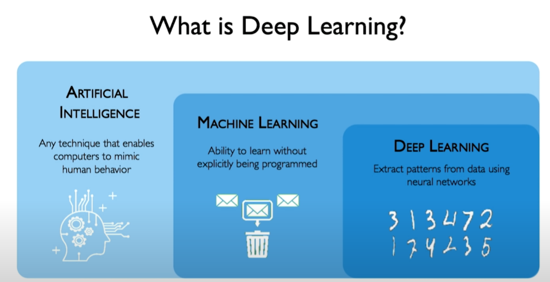
Deep Learning
Cerchiamo innanzitutto di capire cosa è il deep learning e come si relaziona con il machine learning e l'AI.
[](https://cms.marcocucchi.it/uploads/images/gallery/2023-05/3senXtHhgrfwcYsw-screenshot-2023-05-13-152324.png)
Inferenza
L'inferenza è il processo durante il quale viene sottoposto un nuovo set di dati ad un modello che è stato "trainato" precedente.
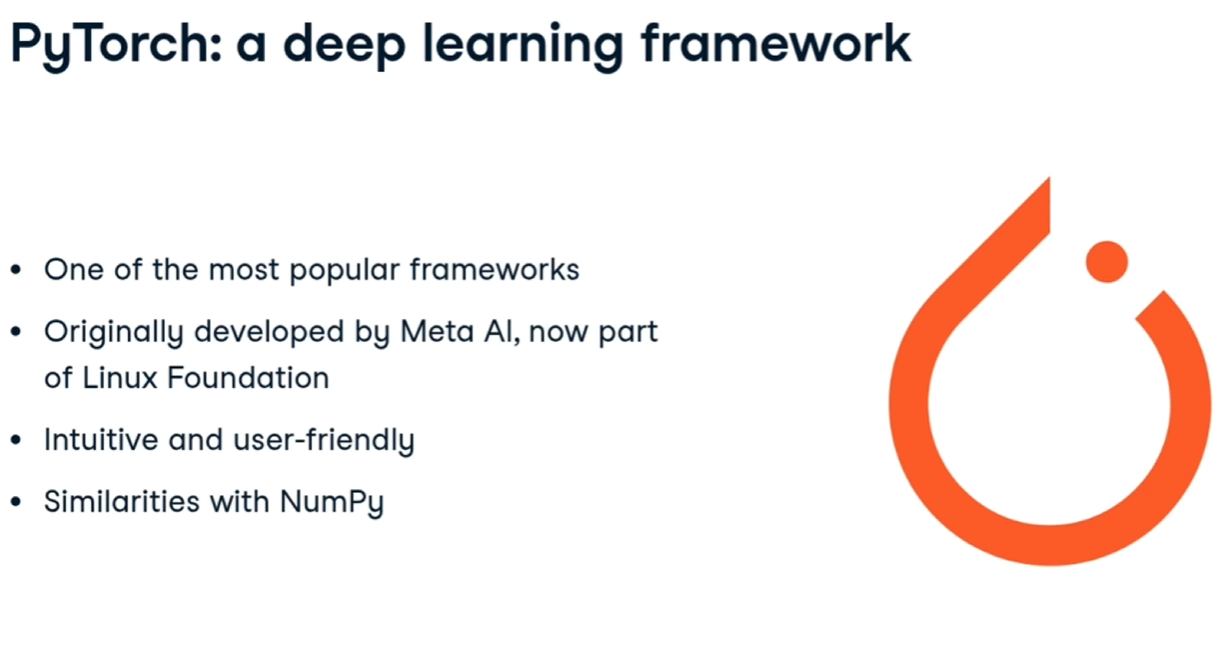
# Pytorch for dummy
[](https://cms.marcocucchi.it/uploads/images/gallery/2025-12/5JInQJzhU0nP5wRP-image.png)
Originariamente impletato da META ora fa parte della Linux foundation
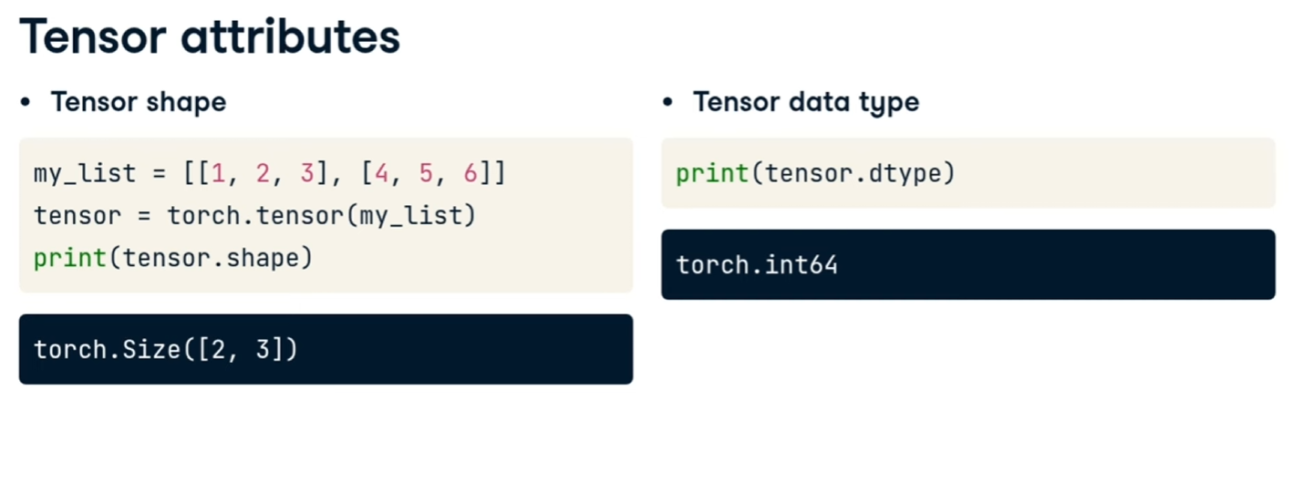
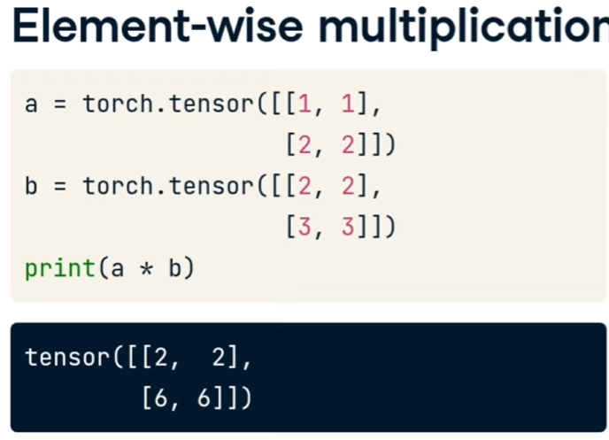
La base di tutto è il tensore, che non è altro che una matrice (o un array) sulla quale PT consente tutta una serie di operazioni, un po' come numpy, es:
[](https://cms.marcocucchi.it/uploads/images/gallery/2025-12/2Wy98ryNFWIMKs54-image.png)
es:
[](https://cms.marcocucchi.it/uploads/images/gallery/2025-12/33x62opLJgWKlLc7-image.png)
##### Layer della rete neurale
[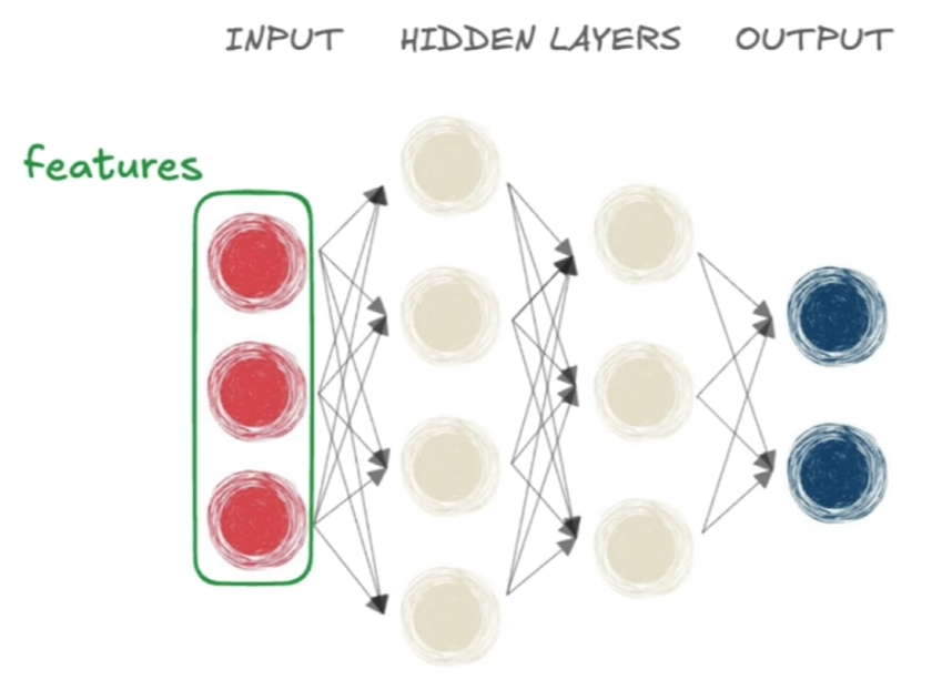](https://cms.marcocucchi.it/uploads/images/gallery/2025-12/GpK546stIUrHPhB4-image.png)
la parte in rosso sono gli input della rete, detta "features", la parte in grigio sono i layer "nascosi", mentra la parte di blu è l'output layer ovvero l'output desiderato.
##### Classificatori
[](https://cms.marcocucchi.it/uploads/images/gallery/2025-12/r2OjVZ9CllxyQQcQ-image.png)
Le funzioni possono essere:
- **Sigmoid** per la classificazione binaria (un unico output con un valore compreso tra 0 e 1)[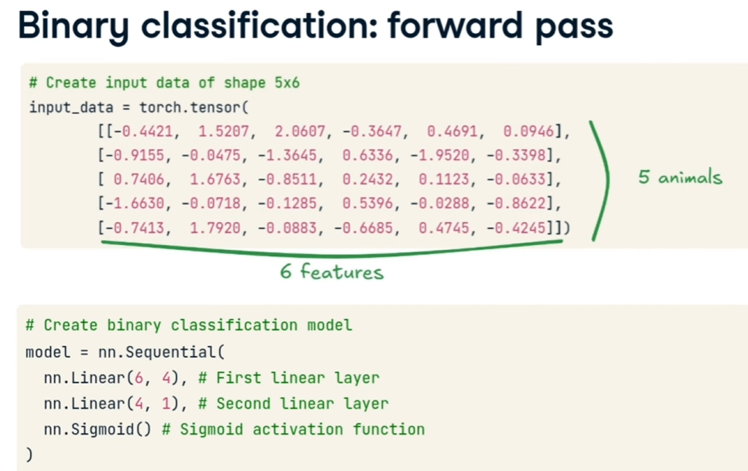](https://cms.marcocucchi.it/uploads/images/gallery/2025-12/Uv23PqcWloLiMdRr-image.png)
- **Softmax** per la multi classificazione, va messo come ultimi layer della rete neurale. (dove l'ultimo livelo di neurino definice il numero di valori da classificre)[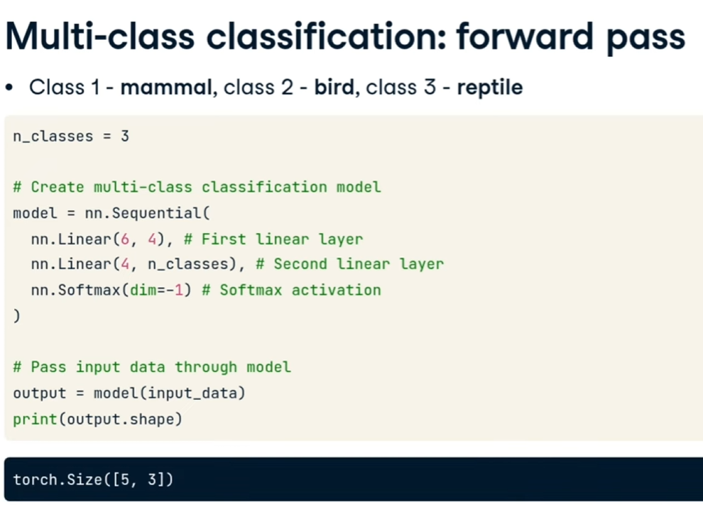](https://cms.marcocucchi.it/uploads/images/gallery/2025-12/zu9mewmoDwJTDmmI-image.png)
- yy per la regressione, ovvero per predirre un flusso continuo di valori numerici, in questo caso non verrò inserita nessuna funzione di attivazione
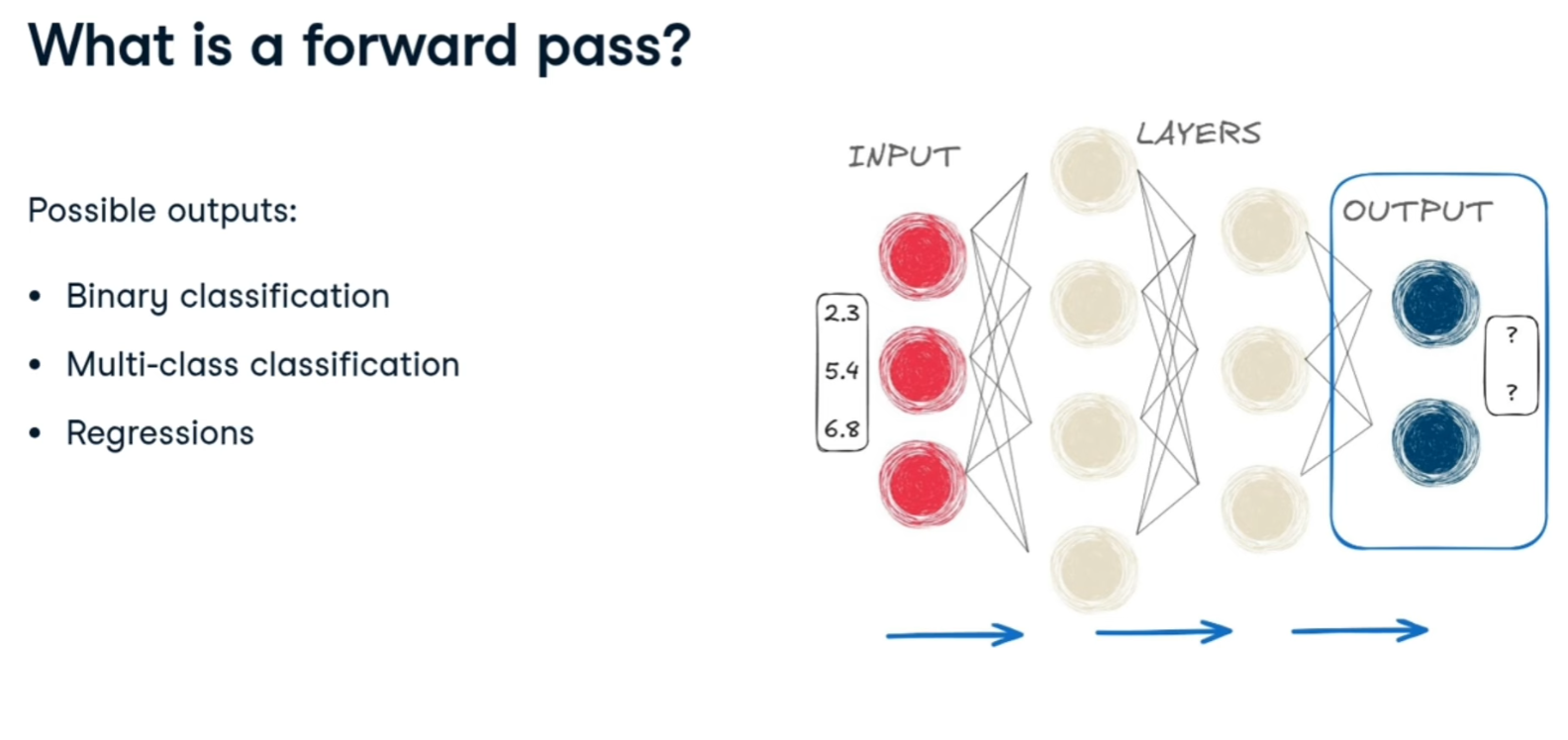
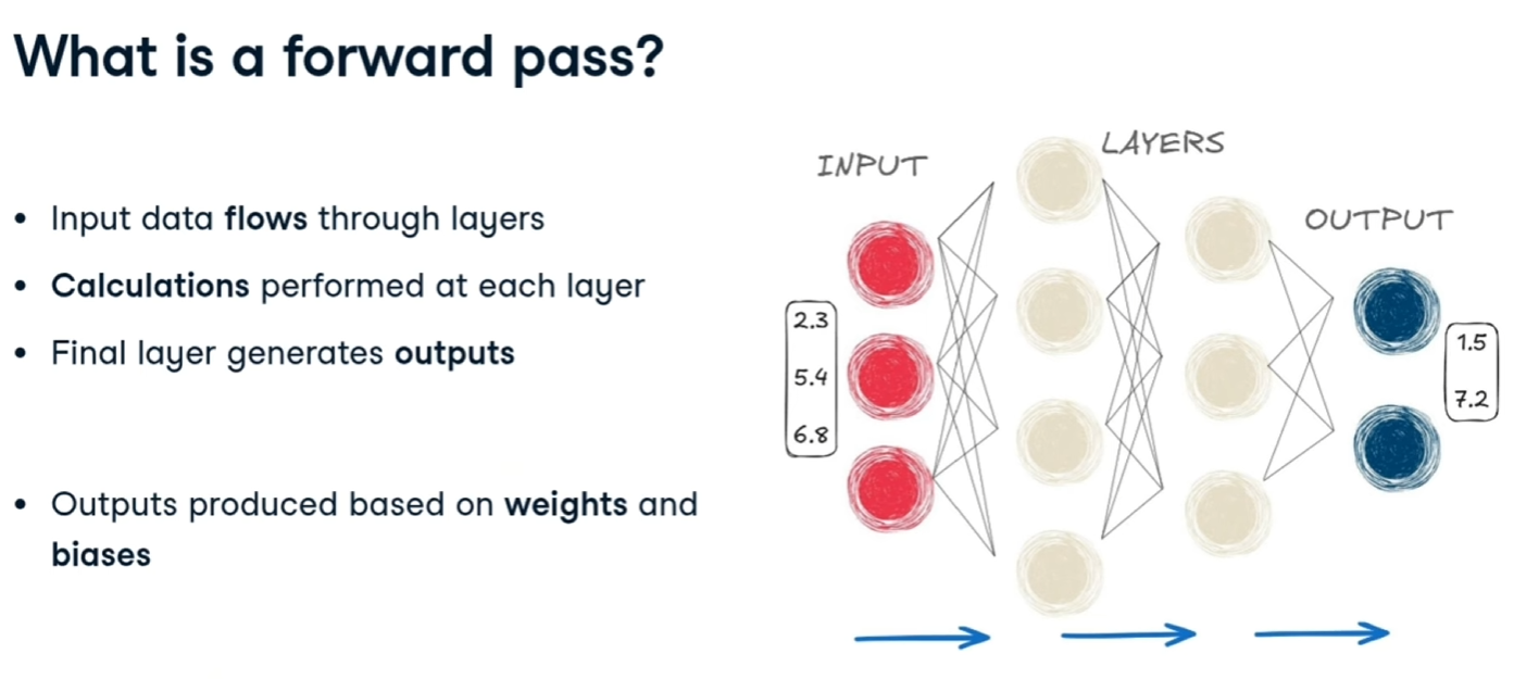
##### Forward pass
è l'operazione di passaggio dei pesi e del bias da un layer della rete a quello successivo
[](https://cms.marcocucchi.it/uploads/images/gallery/2025-12/6Y4LDw7Kmim4FZhM-image.png)
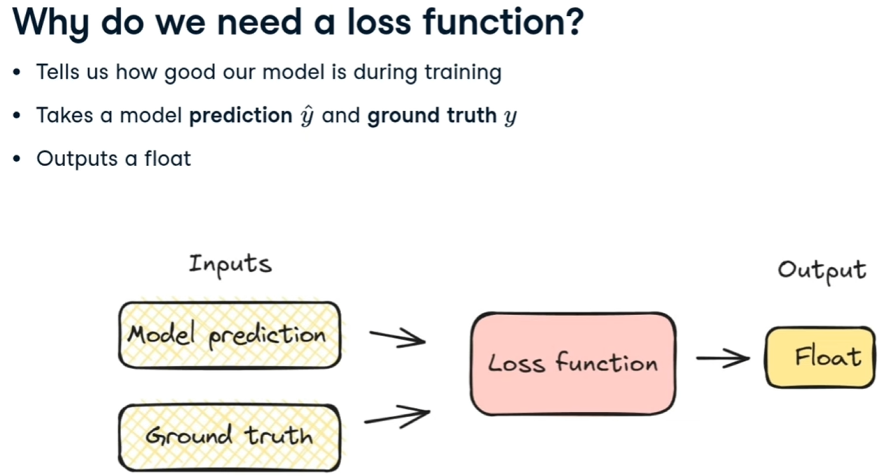
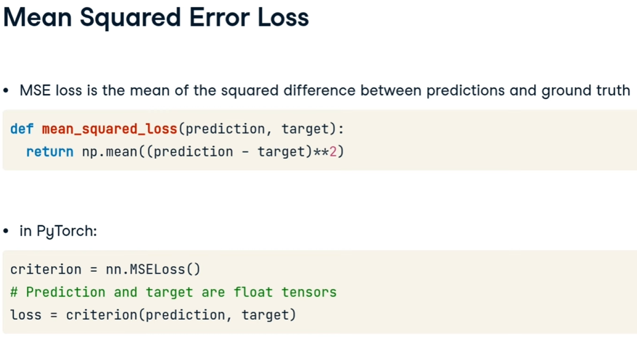
##### Loss function
La LF indica quanto il modello è efficace nel predirre i valori durante la fase di training.
[](https://cms.marcocucchi.it/uploads/images/gallery/2025-12/o97ucS9Qpsjfrtwc-image.png)
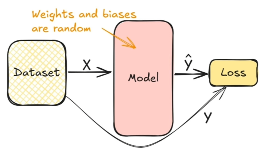
La funzione di "loss" indicata come F, riceve in input i valori corretti associati alle features utilizzate durante il training e quelli generati dal modello -> F(y,**y'**)
L'outuput è un valore numerico
[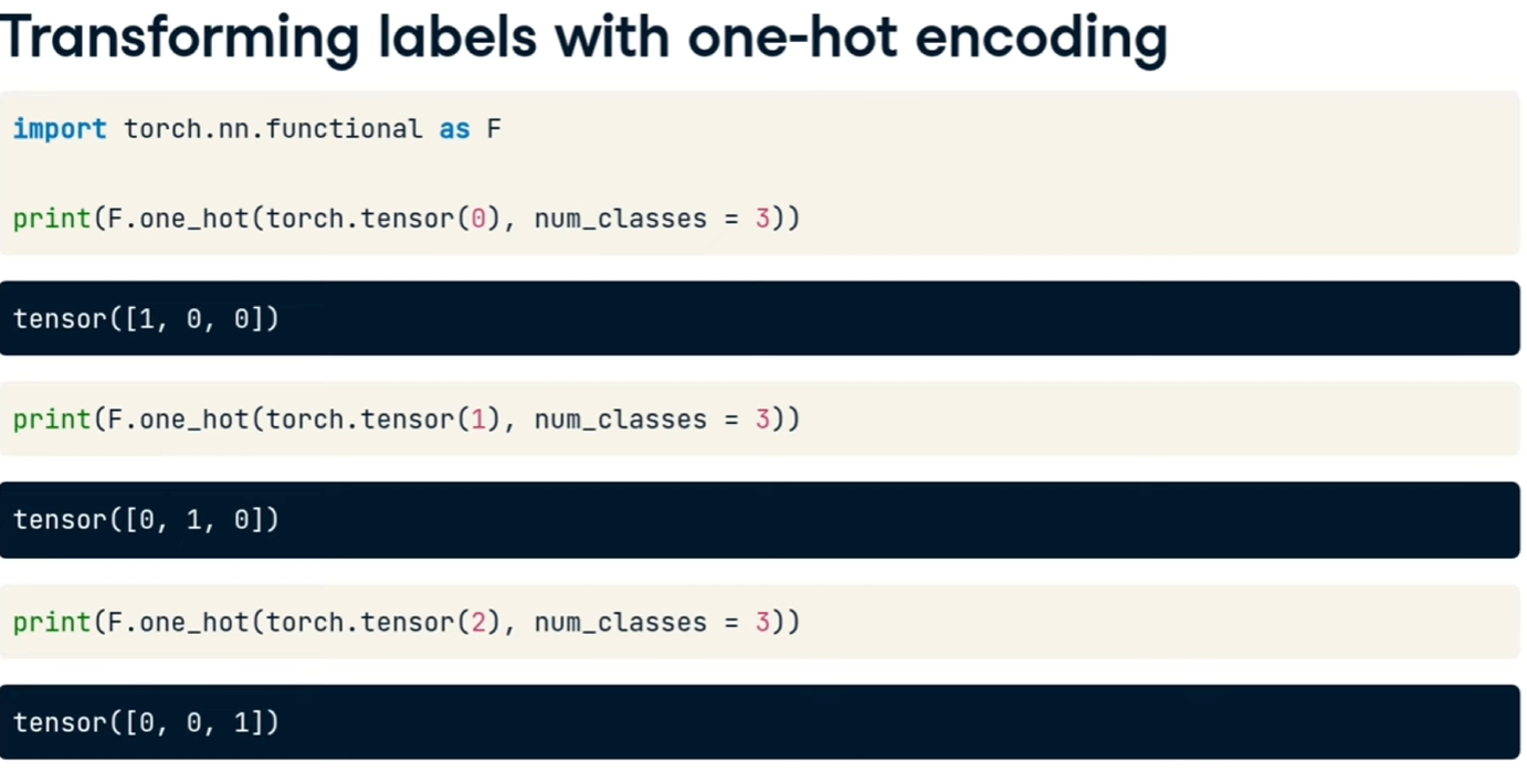](https://cms.marcocucchi.it/uploads/images/gallery/2025-12/TXrs8UtxFNwq4hIk-image.png)
Una delle funzioni di loss function è la *CrossEntropyLoss* che vuole in input i valori calcolati dalla rete e le label che rappresentano il valore "vero". L'ouput è il valore di "**loss**" vero e proprio che, attraverso la backpropagation bisogna minimizzare.
[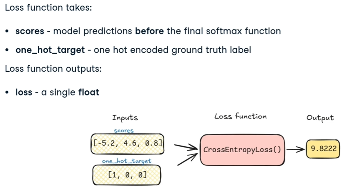](https://cms.marcocucchi.it/uploads/images/gallery/2025-12/hsdvDCYStMh7n3EW-image.png)
#####
[](https://cms.marcocucchi.it/uploads/images/gallery/2025-12/AJwKIZ8go1FVysvq-image.png)
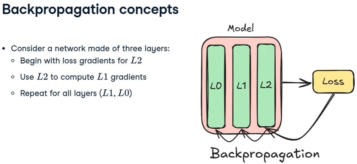
##### La Backpropagation
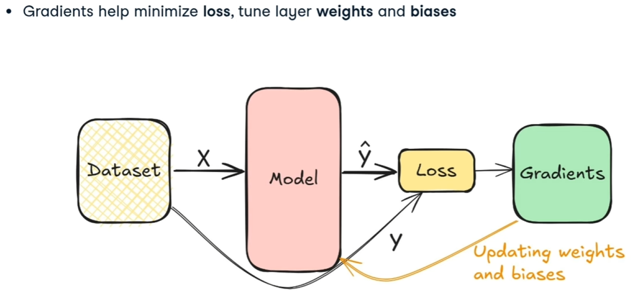
Una volta calcolati i pesi e i bias della rete neurale, si prende il valore generato y' e si effettua un'operazione di backpropagation che, attraverso il calcolo della discesa del gradiente va a ricalcolare i pesi e i bias a ritroso per ciascun layar, al fine dir minimizzare l'errore.
[](https://cms.marcocucchi.it/uploads/images/gallery/2025-12/xYcjFK4yvuWEseUM-image.png)
[](https://cms.marcocucchi.it/uploads/images/gallery/2025-12/vPGF3X9HkRE0FCeM-image.png)
vediamolo in PT:
[](https://cms.marcocucchi.it/uploads/images/gallery/2025-12/GK1IO9UagprJCqVp-image.png)
##### Preparazione dei dati per il training
Ci sono 4 passi fondamentali prima di "allenare" la rete neurale, ovvero:
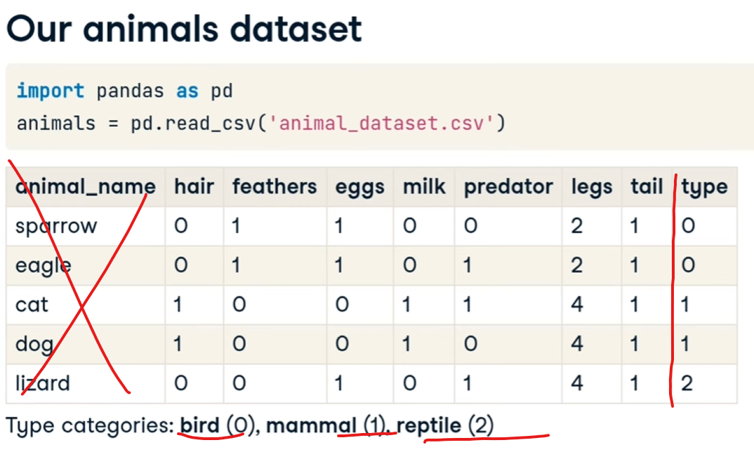
prendiamo per esempio un dataset di animali dove le prime colonne (esclusa la zero che è puramente decrittiva) rappresentano le "features" mentre l'ultima indica il tipo di animale:
[](https://cms.marcocucchi.it/uploads/images/gallery/2025-12/QTiG2tdyTBJIUXIi-image.png)
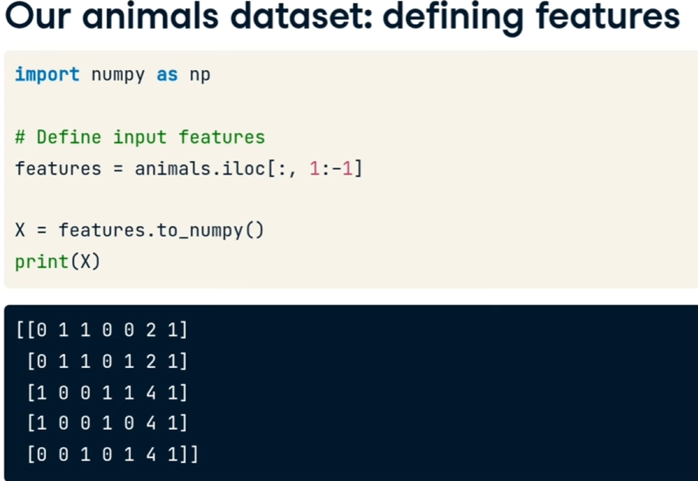
selezioniamo le fetures:
[](https://cms.marcocucchi.it/uploads/images/gallery/2025-12/AKgS39O4CBVDEKH5-image.png)
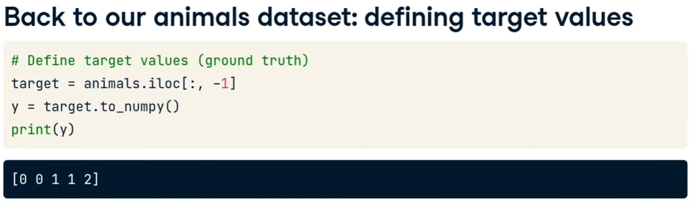
ora le labels
[](https://cms.marcocucchi.it/uploads/images/gallery/2025-12/HGmzTqnF98qIwZvJ-image.png)
Ora utilizziamo l'oggetto TensorDataset per caricare le x e le y:
[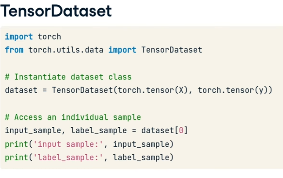](https://cms.marcocucchi.it/uploads/images/gallery/2025-12/VrGMWIQdANcPflta-image.png)
ora creiamo il dataloader per gestire il carico dei dati efficacemente durante il training
[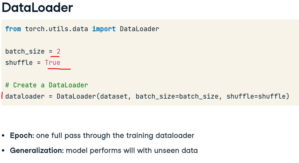](https://cms.marcocucchi.it/uploads/images/gallery/2025-12/Guz5Igol1Y9amfR2-image.png)
avendo setto il batch size a 2 ad ogni iterazione del dataloader estrarrò solo un bach di due elementi (in questo 2 carratteristiche di animali e il tipo), come sotto riportato:
[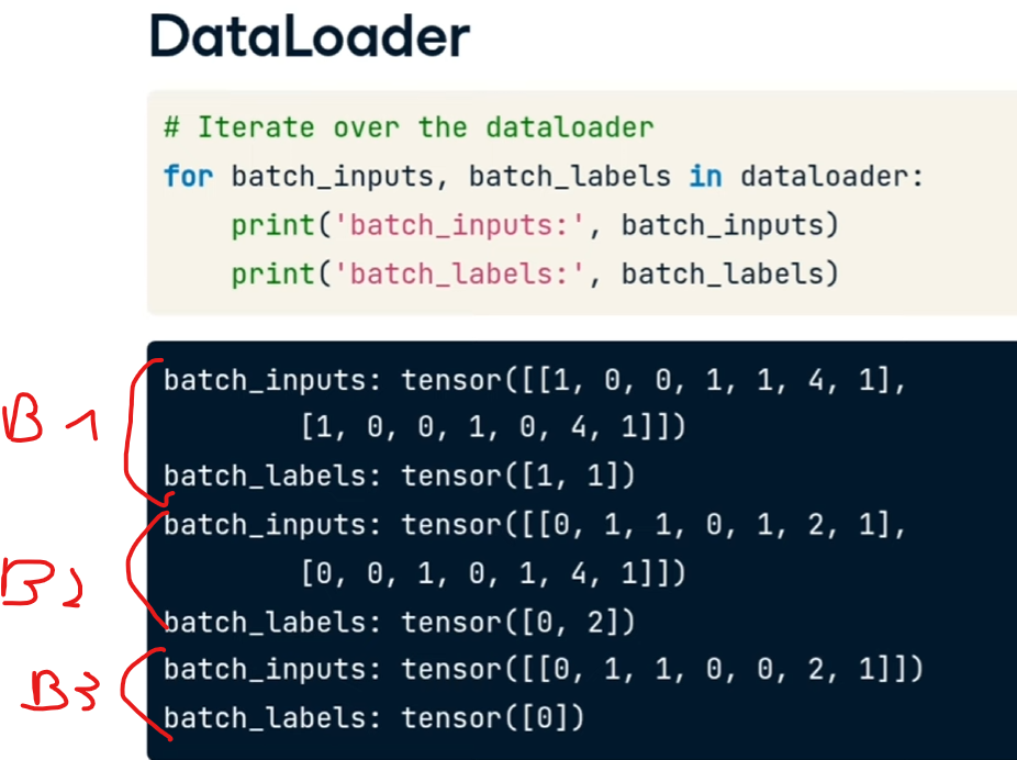](https://cms.marcocucchi.it/uploads/images/gallery/2025-12/5AW7N3Uczgje0T3m-image.png)
essemdo solo 5 animali si può notarer come l'ultimo batch contenga un solo animale.
**Quindi il cliclo for fa passare tutto il dataset.**
##### Training
ora possiamo procedere con il training, che consiste in:
[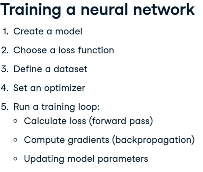](https://cms.marcocucchi.it/uploads/images/gallery/2025-12/Eh6m7MKLaLRpBso9-image.png)
Il training è molto importante perchè consenti di minimizzare la loss e di appore delle modifiche al training stesso.
##### Regressione
La regressione consente di avere un valore lineare come output.
Per la regressione so utilizza in genere la funzione di loss MSE (mean square error)
[](https://cms.marcocucchi.it/uploads/images/gallery/2025-12/0HVVwCmCm9JndKAx-image.png)
facciamo un esempio di regression i gli stipendi dei data scientist:
[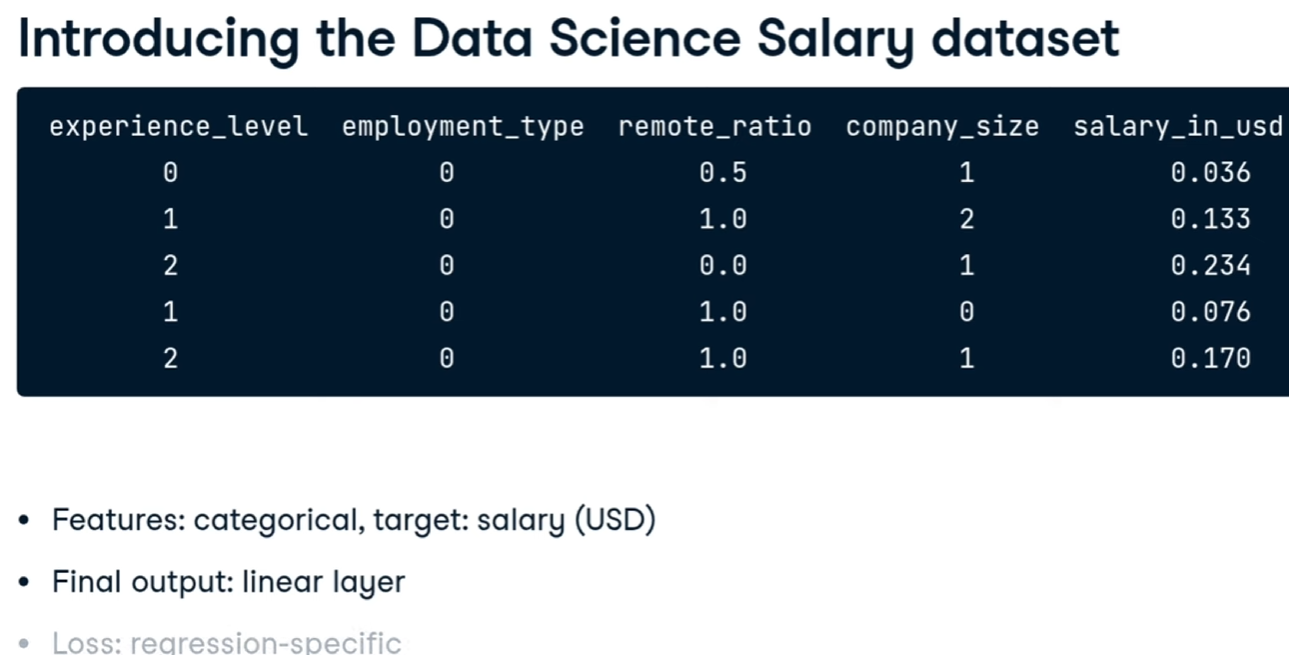](https://cms.marcocucchi.it/uploads/images/gallery/2025-12/utNvjH8uVVlTeSX3-image.png)
creiamo la rete neurale
[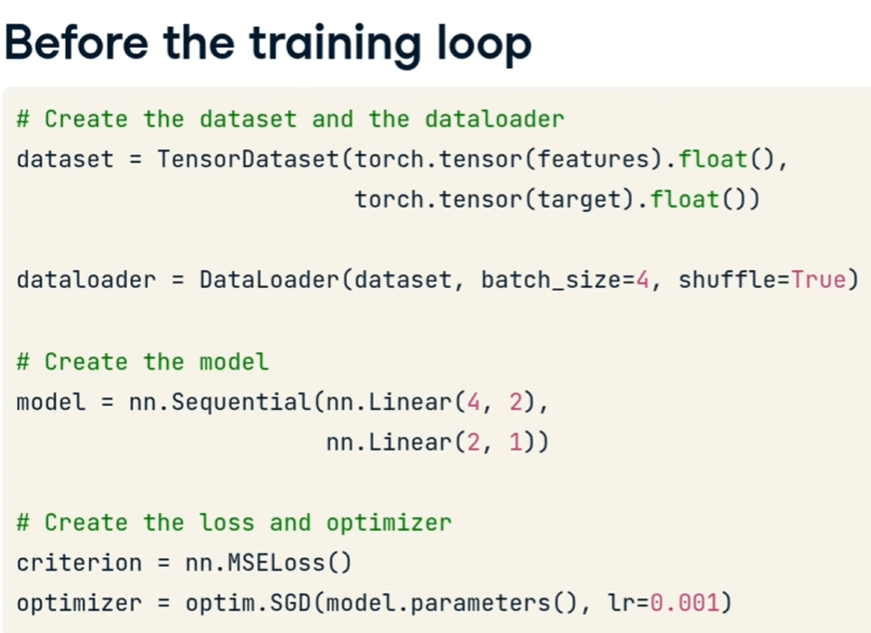](https://cms.marcocucchi.it/uploads/images/gallery/2025-12/PnwueCqqq9gXnyND-image.png)
adesso loppiamo su tutto il dataset
```python
# The training loop
for epoch in range(num_epochs):
for data in dataloader:
# va azzerato ad ogni epoca
optimizer.zero_grad()
# Get feature and target from the data loader
feature, target = data
# Run a forward pass
pred = model(feature)
# Compute loss and gradients
loss = criterion(pred, target)
loss.backward()
# Update the parameters
optimizer.step()
```
##### Utilizzo Softmax vs ReLU.
E' emerso che per gli hidden layer è meglio utilizzare la **funzione di attivazione** ReLU, mentre per l'output layer si può utilizzare anche la Softmax.
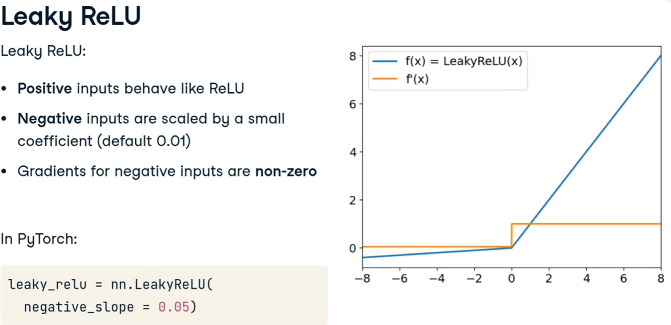
##### Leaky ReLU
Migliora la ReLU moltiplicando i valori di input per un coefficiente che evita i casi di disattivazione totale del neurone che causa lo stop dell'apprendimento.
[](https://cms.marcocucchi.it/uploads/images/gallery/2025-12/xGDkPzkRsuMfHqIC-image.png)
##### Learing rate e momentum
Il LR è il passo utilizzato per arrivare al mimimo durante la fase della discesa del gradiente, se è troppo piccolo non arrivieremo al minimo, come qui:
[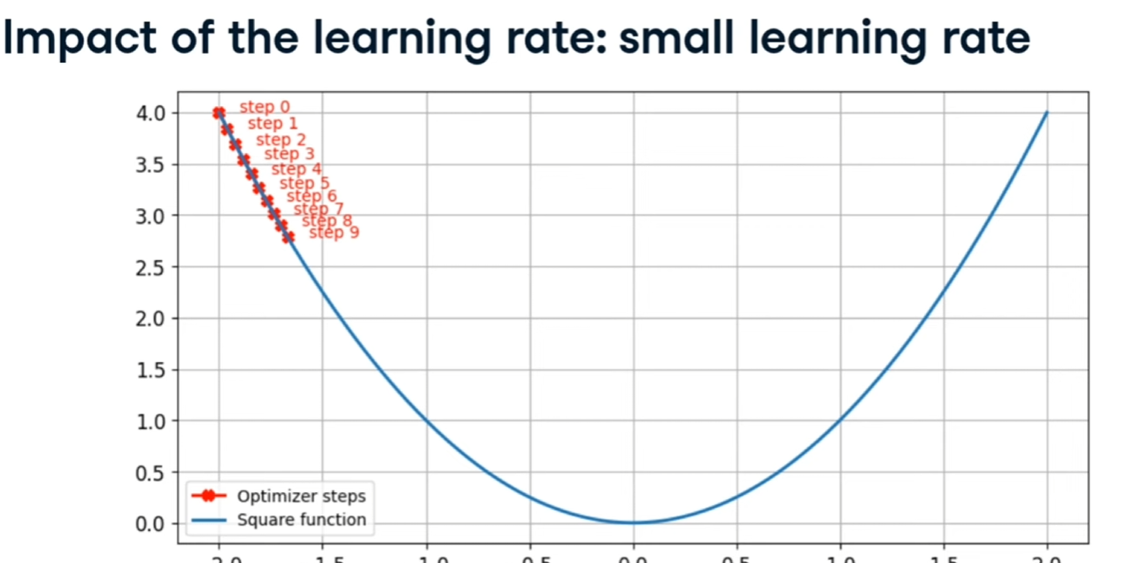](https://cms.marcocucchi.it/uploads/images/gallery/2025-12/OFYUV1WRvZI3PCoL-image.png)
se è troppo grande, continua a rimbalzare senza trovare cmq il minimo, come qui:
[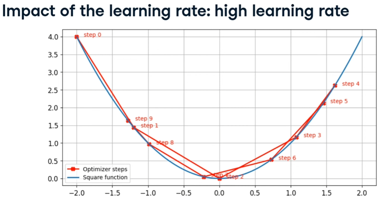](https://cms.marcocucchi.it/uploads/images/gallery/2025-12/JVJouDcm27ScueSC-image.png)
Il "momento" invece rappresenta l'inzeria con la quale si effettuano i passi, serve per evitare di fermarsi ad un "minimo locale", in sintesi:
[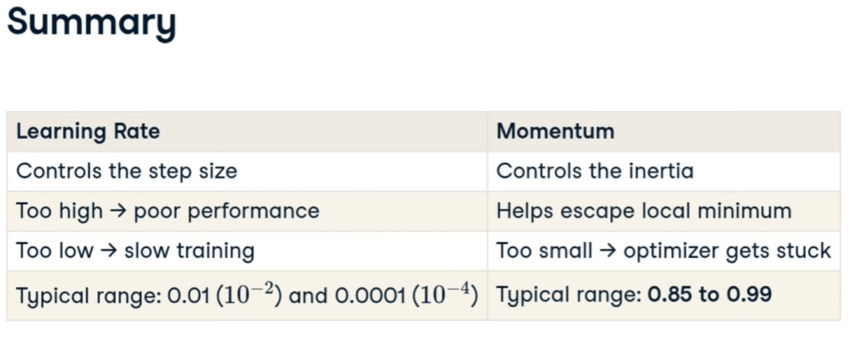](https://cms.marcocucchi.it/uploads/images/gallery/2025-12/UuSxqfXQ6EjVQZwL-image.png)
Valutazione del modello
https://www.youtube.com/watch?v=IFsVsXAqPto
[47:37](https://www.youtube.com/watch?v=IFsVsXAqPto&t=2857s) Evaluating Models with Training and Validation Data
# Tensore
#### Cosa è un tensore?
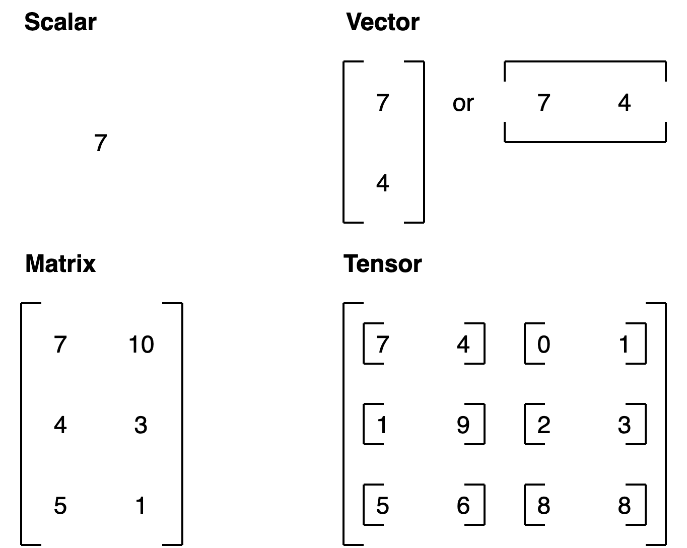
Il tensore è uno scalare (valore singolo), un vettore o una matrice multidimensionale, nella quale vengono storati i valori utilizzati da pytorch.
Nella pratica un tensore è la rappresntazione numerica in forma di array/matrici di un qualsiasi fenomeno esterno, sia esso per es. un'immagine, un suono o un range di valori numerici.
es:
```python
# Scalar
cuda0 = torch.device('cuda:0')
scalar = torch.tensor(7, device=cuda0)
scalar
```
In questo caso istanzio uno scalare contenete il valore 7, da notere che, avendo un GPU vado a storare questo valore nella ram del GPU e non della cpu.
Di seguito un esempio di matrice
```python
MATRIX = torch.tensor([[7, 8],
[9, 10]], device=cuda0)
MATRIX
```
[](https://cms.marcocucchi.it/uploads/images/gallery/2022-12/vURm1G8iHvSJKpvI-00-scalar-vector-matrix-tensor.png)
##### Le dimensioni del tensore
[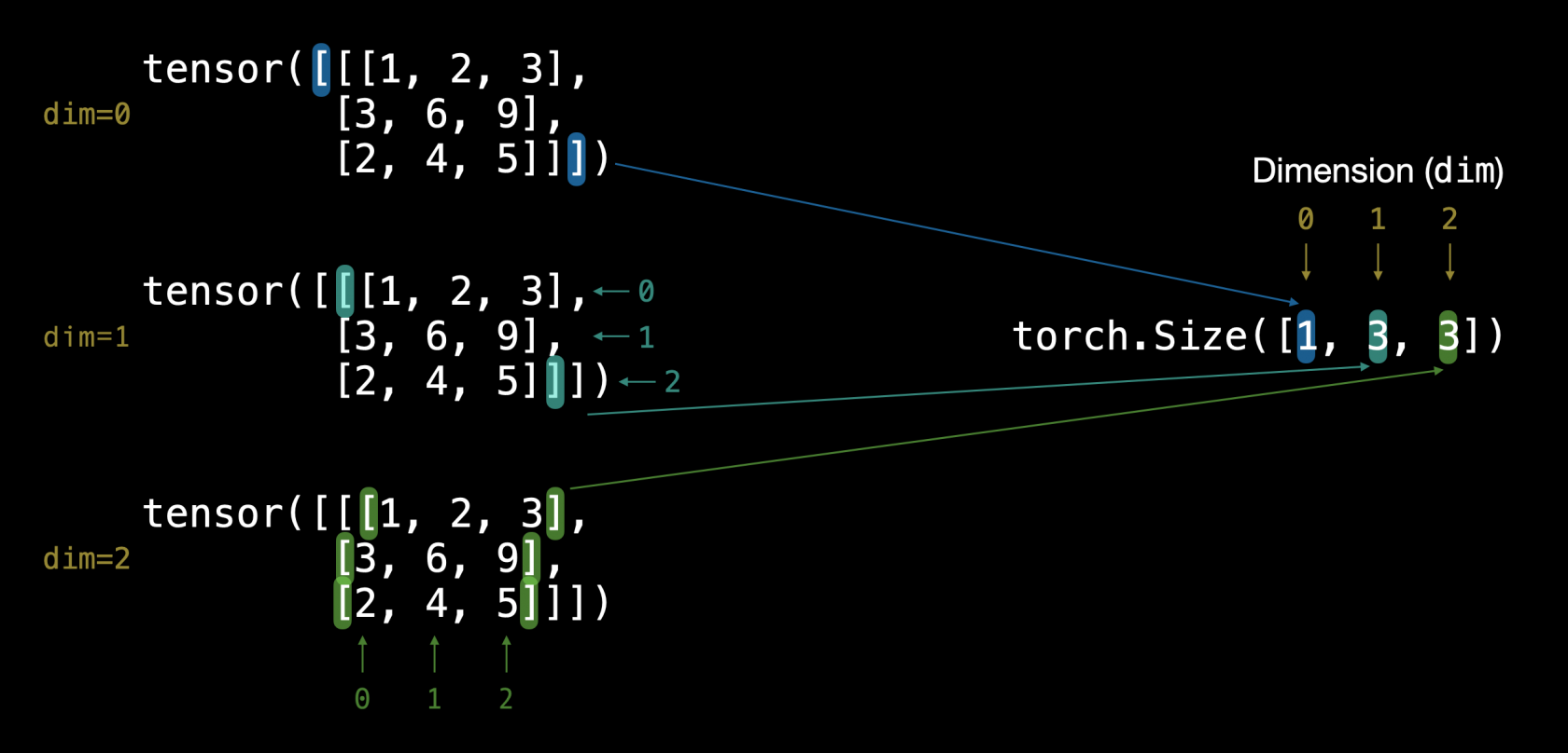](https://cms.marcocucchi.it/uploads/images/gallery/2023-01/axGhsOdefd0umYN4-00-pytorch-different-tensor-dimensions.png)
**NB**: cerchiamo di capire bene la differenza tra la dimention e la size. La dimension indica quanti livelli "innestati" sono definiti all'interno della matrice, mentre la size indica il numero totali di righe-colonne presenti nella matrice.
##### Tensori randomici
Sono molto utili nelle fasi iniziali del training , di seguito un esempio per la creazione:
```python
random_tensor = torch.rand(3,4)
tensor([[0.1207, 0.8136, 0.9750, 0.5804],
[0.4229, 0.6942, 0.4774, 0.5260],
[0.2809, 0.1866, 0.8354, 0.7496]])
# oppure altro esempio:
import torch
cuda0 = torch.device('cuda:0')
random_tensor = torch.rand(2,3,4, device=cuda0)
print (random_tensor)
tensor([[[0.2652, 0.6430, 0.7058, 0.3049],
[0.3983, 0.4169, 0.6228, 0.6622],
[0.6239, 0.7246, 0.1134, 0.9273]],
[[0.5454, 0.9085, 0.2009, 0.7056],
[0.5211, 0.6397, 0.9299, 0.1871],
[0.8542, 0.1733, 0.4378, 0.3836]]], device='cuda:0')
# dove si evince il tensore è di 2 righe ciascuna delle quali è composta
# a sua volta da una matri di 3 righe per 4 colonne
```
se invce si vuole crare un tensore di zeroes.
zeros = torch.zeros(size=(3, 4))
##### Range di tesori
```python
Use torch.arange(), torch.range() is deprecated
zero_to_ten_deprecated = torch.range(0, 10) # Note: this may return an error in the future
# Create a range of values 0 to 10
zero_to_ten = torch.arange(start=0, end=10, step=1)
print(zero_to_ten)
> tensor([0, 1, 2, 3, 4, 5, 6, 7, 8, 9])
```
se vuole creare un tensore che la le stesse dimensioni di un altro
```python
ten_zeros = torch.zeros_like(input=zero_to_ten) # will have same shape
print(ten_zeros)
```
##### DTypes
è il datatype che definisce i dati contenuto nel tensore
per vedere i tipi di datatypes: [https://pytorch.org/docs/stable/tensors.html#data-types](https://pytorch.org/docs/stable/tensors.html#data-types)
```python
# Default datatype for tensors is float32
float_32_tensor = torch.tensor([3.0, 6.0, 9.0],
dtype=None, # defaults to None, which is torch.float32 or whatever datatype is passed
device=None, # defaults to None, which uses the default tensor type
requires_grad=False) # if True, operations perfromed on the tensor are recorded
float_32_tensor.shape, float_32_tensor.dtype, float_32_tensor.device
# Create a tensor
some_tensor = torch.rand(3, 4)
# Find out details about it
print(some_tensor)
print(f"Shape of tensor: {some_tensor.shape}")
print(f"Datatype of tensor: {some_tensor.dtype}")
print(f"Device tensor is stored on: {some_tensor.device}") # will default to CPU
tensor([[0.2423, 0.6624, 0.3201, 0.3021],
[0.7961, 0.9539, 0.0791, 0.8537],
[0.3491, 0.6429, 0.8308, 0.4690]])
Shape of tensor: torch.Size([3, 4])
Datatype of tensor: torch.float32
Device tensor is stored on: cpu
```
***Forzare i tipi***
Ovviamente è possibile cambiare il dtype per quei casi in cui le operazioni generano degli errori per es.
x = torch.arange(0,100,10)
print (x, x.dtype)
> tensor([ 0, 10, 20, 30, 40, 50, 60, 70, 80, 90]) torch.int64
ma la funzione media non accetta un tipo "long" per cui dovremmo formare il vettore a float come sotto riportato:
y= torch.mean(x.type(torch.float32))
print(y)
oppure
print( x.type(torch.float32).mean() )
>tensor(45.)
##### Operazioni con i tensori
NB: nelle operazioni con i tensori, es. le moltiplicazioni, posso effettuarle tra tipi diversi. (es. int16 x float32)
Le operazioni basi sono le classiche: +,-,\*,/ e moltiplicazione tra matrici:
```python
# Create a tensor of values and add a number to it
tensor = torch.tensor([1, 2, 3])
tensor + 10
tensor([11, 12, 13])
# Multiply it by 10
tensor * 10
tensor([10, 20, 30])
#Notice how the tensor values above didn't end up being tensor([110, 120, 130]), this is because the values inside the tensor don't
#change unless they're reassigned.
# Tensors don't change unless reassigned
tensor
tensor([1, 2, 3])
#Let's subtract a number and this time we'll reassign the tensor variable.
# Subtract and reassign
tensor = tensor - 10
tensor
tensor([-9, -8, -7])
# Add and reassign
tensor = tensor + 10
tensor
tensor([1, 2, 3])
PyTorch also has a bunch of built-in functions like torch.mul() (short for multiplcation) and torch.add() to perform basic operations.
# Can also use torch functions
torch.multiply(tensor, 10)
tensor([10, 20, 30])
# Original tensor is still unchanged
tensor
tensor([1, 2, 3])
#However, it's more common to use the operator symbols like * instead of torch.mul()
# Element-wise multiplication (each element multiplies its equivalent, index 0->0, 1->1, 2->2)
print(tensor, "*", tensor)
print("Equals:", tensor * tensor)
tensor([1, 2, 3]) * tensor([1, 2, 3])
Equals: tensor([1, 4, 9])
```
Moltiplicazione tra matrici
One of the most common operations in machine learning and deep learning algorithms (like neural networks) is [matrix multiplication](https://www.mathsisfun.com/algebra/matrix-multiplying.html).
PyTorch implements matrix multiplication functionality in the [`torch.matmul()`](https://pytorch.org/docs/stable/generated/torch.matmul.html) method.
**Regole della moltiplicaazione di matrici**
***Regola della dimensione interna***
La dimensione **interna DEV**E essere la stessa, ovvero, se abbiamo una matrice (3,2) e un'altra matrice di (3,2)
la moltiplicazione genererà un errore in quanto le dimensioni interne non coincidono.
Per dimensione interna si intende (3,**2**) x (**2**,3) in questo caso il 2, dove nella prima matricie sono le colonne mentre nella secondo le righe. (nel primo esempio erano invece diverse e quindi non è possibile effettuare la moltiplicazione.
***Regola della matrice risultante***
La shape della matrice risultante è **pari alle dimensini esterne** delle due matrici.
Ovvero nel caso di matrici (2,3) x (3,2) che quindi soffisfano la regola della dimensione interna, la risultante sarà una matrice la cui dimensione sarà la dimensione esterna, quindi (2,2)
***Come moltiplicare due matrici***
Di seguito viene mostrato graficamente come moltiplicare due matrici:
[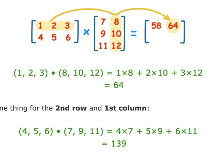](https://cms.marcocucchi.it/uploads/images/gallery/2023-01/wdTNBXvtvF7EWb8g-screenshot-2023-01-01-111502.png)
....
[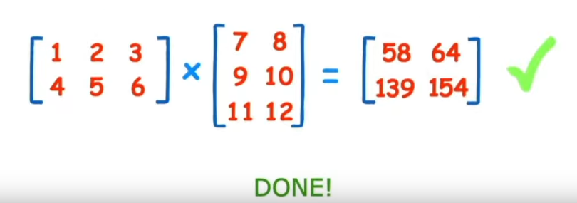](https://cms.marcocucchi.it/uploads/images/gallery/2023-01/A4DZGsuDHknbV6tG-screenshot-2023-01-01-111502.png)
Differenza tra "**Element-wise multiplication"** e "**Matrix multiplication"**.
Element wise moltiplication moltiplica ogni elemento mentre invece matrix multiplication effettua il totale delle moltiplicatione delle matrici.
`tensor` variable with values `[1, 2, 3]`:
| Operation | Calculation | Code |
|---|
| \*\*Element-wise multiplication\*\* | `\[1\*1, 2\*2, 3\*3\]` = `\[1, 4, 9\]` | `tensor \* tensor` |
| \*\*Matrix multiplication\*\* | `\[1\*1 + 2\*2 + 3\*3\]` = `\[14\]` | `tensor.matmul(tensor)` |
```python
# Element-wise matrix multiplication
tensor * tensor
>tensor([1, 4, 9])
# Matrix multiplication
torch.matmul(tensor, tensor)
> tensor(14)
# Can also use the "@" symbol for matrix multiplication, though not recommended
tensor @ tensor
>tensor(14)
```
#### Manipolazione dello shape
Coonsideriamo il caso
```python
tensor_A = torch.tensor([[1, 2],
[3, 4],
[5, 6]], dtype=torch.float32)
tensor_B = torch.tensor([[7, 10],
[8, 11],
[9, 12],
[13,14]], dtype=torch.float32)
```
se eftettuiamo la motiplicazione dei due, per le due regole sopra citate, verrà generato un errore in quanto la dimensione interna non matcha:
errore -> torch.matmul(tensor\_A, tensor\_B) in quanto abbiamo una moltiplicare di (3,2) x (4,2) che non coincidono internamente.
ma allora che fare? ebbene in questo caso possiamo far coincidere le dimensioni interne di uno dei due tensori utilizzando la funzione "transpose", come di seguito
torch.matmul(tensor\_A, tensor\_B**.T**) dove il metodo .T effettua la traspose del tensore B rendendolo compatibile con A, ovvero:
```
tensor([[ 7., 8., 9., 13.],
[10., 11., 12., 14.]])
```
che traspone la (4,2) in (2,4) e quindi l'output della moltiplicare sarà:
```
# effetto la moltiplicazione ora con la transposizione è diventato -> torch.Size([3, 2]) * torch.Size([2, 4])
torch.mm(tensor_A*tensor_A.T)
Output:
tensor([[ 27., 30., 33., 41.],
[ 61., 68., 75., 95.],
[ 95., 106., 117., 149.]])
Output shape: torch.Size([3, 4])
```
che soddispafa la prima regola (dimensione interna) e la seconda regola (dimensione tensore risultate pari alla dimensione esterna)
NOTA: per fare delle prove andare sul sito [http://matrixmultiplication.xyz/](http://matrixmultiplication.xyz/)
##### Aggregazione del tensore
Oltre alla moltiplicazione abbiamo altri tipi di operazioni comuni che possono essere effettuate sui tensori ovvero:
min, max, mean, sum, ed altro... che nella pratica si tratta di invocare il metodo dell'oggetto "torch" es. torch.mean(tensore)
**NOTA**: Può essere che questi metodi diano degli errori sui tipi, es il metodo mean non accetta un dtype long, per questo motivo il tipo può essere convertito "al volo" tramite il metodo type, es. torch.mean ( X.type(torch.float32) ) -> che lo casta a floating 32.
##### Posizionamento del min e del max
Se vogliamo sapere l'indice del valore minimo o massimo all'iterno del tensore allora toch ci mette a disposizione il metodo argmin es.
```python
#Create a tensor
tensor = torch.arange(10, 100, 10)
print(f"Tensor: {tensor}")
# Returns index of max and min values
print(f"Index where max value occurs: {tensor.argmax()}")
print(f"Index where min value occurs: {tensor.argmin()}")
Tensor: tensor([10, 20, 30, 40, 50, 60, 70, 80, 90])
Index where max value occurs: 8
Index where min value occurs: 0
```
#### Reshaping, stacking, squeezing e un squeezing
Lo scopo di questi metodi è manipolare il tensore in modo da modificarne lo "shape" o la dimensione. Di seguito viene riportata una breve descrizione dei metodi.
| Metodo | Descrizione (online) |
|---|
| [torch.reshape(input, shape)](https://pytorch.org/docs/stable/generated/torch.reshape.html#torch.reshape) | Reshapes `input` to `shape` (if compatible), can also use `torch.Tensor.reshape()`. |
| [torch.Tensor.view(shape)](https://cms.marcocucchi.it/(https:/pytorch.org/docs/stable/generated/torch.Tensor.view.html) | Returns a view of the original tensor in a different `shape` but shares the same data as the original tensor. |
| [torch.stack(tensors, dim=0)](https://pytorch.org/docs/1.9.1/generated/torch.stack.html) | \*\*Concatenates\*\* a sequence of `tensors` along a new dimension (`dim`), all `tensors` must be same size. |
| [torch.squeeze(input)](https://pytorch.org/docs/stable/generated/torch.squeeze.html) | Squeezes `input` to \*\*remove\*\* all the dimenions with value `1`. |
| [torch.unsqueeze(input, dim)](https://pytorch.org/docs/1.9.1/generated/torch.unsqueeze.html) | Returns `input` with a dimension value of `1` \*\*added\*\* at `dim`. |
| [torch.permute(input, dims)](https://pytorch.org/docs/stable/generated/torch.permute.html) | Returns a \*view\* of the original `input` with its dimensions permuted (rearranged) to `dims`. |
creiamo un vettore con 9 valori:
```
# creo un vettore semplice
import torch
x = torch.arange(1., 10.)
x, x.shape
tensor([1., 2., 3., 4., 5., 6., 7., 8., 9.])
shape -> torch.Size([9])
```
##### Reshape
Nell'esempsio voglio convertire il tensore in una matrice di una riga per nove colonne, visto che il numero di elementi è compatibile con l'operazione.
**ATTENZIONE** che reshape deve essere compatibile con la dimensione.
Quindi:
y = x.reshape(9,1)
y varrà:
```
tensor([[1.],
[2.],
[3.],
[4.],
[5.],
[6.],
[7.],
[8.],
[9.]])
shape -> torch.Size([9, 1])
```
se inceve volessimo creare un tensore multidimensionale di una riga per nove colonne:
y = x.reshape(1,9)
``` tensor(\[\[1., 2., 3., 4., 5., 6., 7., 8., 9.\]\])
shape -> torch.Size(\[1, 9\])
```
##### View
La view è simile a reshape solo che l'output condivide la stessa area di memoria, in pratica modificando uno si modifica anche l'altro, es.
z = x.view(1,9)
\# questo comando modifica la colonna zero di tutte le righe (vale anche se abbiamo una sola riga)
z \[:,0\] = 5
a questo punto sia z che x puntano allo stesso valore (5) nella colonna zero
##### Stack
Concatena due o più tensori purchè abbiano la stessa dimensione e che siano in una lista. (es.
```python
tensor_one = torch.tensor([[1,2,3],[4,5,6]])
print(tensor_one)
tensor([[1, 2, 3],
[4, 5, 6]])
tensor_two = torch.tensor([[7,8,9],[10,11,12]])
tensor_tre = torch.tensor([[13,14,15],[16,17,18]])
#NB devono essere in una lista es. tensor_list = [tensor_one, tensor_two, tensor_tre] o direttamente come sotto
staked_tensor = torch.stack([tensor_one,tensor_two,tensor_tre])
print(staked_tensor.shape)
torch.Size([3, 2, 3])
print(staked_tensor)
tensor([[[ 1, 2, 3],
[ 4, 5, 6]],
[[ 7, 8, 9],
[10, 11, 12]],
[[13, 14, 15],
[16, 17, 18]]])
```
##### Squeeze e UnSqueeze
Lo squeeze rimuove tutte le dimensioni "singole" dal tensore, es:
```python
import torch
# creo un array a (dimensione 0)
xx = torch.arange(1., 10.)
print (xx)
>tensor([1., 2., 3., 4., 5., 6., 7., 8., 9.])
# aggiungo una dimensione (dimensione 1)
xx = xx.reshape(1,9)
print (xx)
>tensor([[1., 2., 3., 4., 5., 6., 7., 8., 9.]])
#tolgo la dimensione che ho aggiunto (solo se dim 1)
print(xx.squeeze())
print (xx)
>tensor([1., 2., 3., 4., 5., 6., 7., 8., 9.])
#Con l'unsqueeze si aggiunga una singola dimensione
print(staked_tensor.squeeze())
>tensor([[[1., 2., 3., 4., 5., 6., 7., 8., 9.]]])
```
##### Permute
L'operazione permute permette di "switchare" una dimensione con l'altra, ovvero:
```python
# creiamo un tensore di dimensione 3 di 224 x 224 x 3, che btw potrebbe
# rappresentare un'immagine dove le prime due dimensione sono i pixel mentre la terza il valore RGB
x_original = torch.rand(size=(224, 224, 3))
# la permute lavora per indici, nel caso specifico swppiamo il secondo indice ( è zero based) e lo
# mettimao al primo posto (zero) e così via
x_permuted = x_original.permute(2, 0, 1) # shifts axis 0->1, 1->2, 2->0
print(f"Previous shape: {x_original.shape}")
Previous shape: torch.Size([224, 224, 3])
print(f"New shape: {x_permuted.shape}")
New shape: torch.Size([3, 224, 224])
si noti quindi i valori delle dimensioni vengono "swappati" tra di loro secondo l'ordine definito dal medoto "permute"
ricordarsi inoltre che anche la permute lavora su una vista dei valori originali, con tutto ciò che comporta l'uso di una vista in torch
```
##### Indexing
L'indexing è utilizzato per estrapolare, navigare, i dati di un tensore, con pytorch è simile a quello di numpy.
es.
\# Creo un tensore
```python
import torch
x = torch.arange(1, 10).reshape(1, 3, 3)
x, x.shape
>tensor([[[1, 2, 3],
[4, 5, 6],
[7, 8, 9]]]
>torch.Size([1, 3, 3])
# target su primo elemento della matrice tridimensionale
x[0]
>tensor([[1, 2, 3],
[4, 5, 6],
[7, 8, 9]])
# target su primo elemento della matrice tridimensionale e di questo elemento il primo
x[0][0]
>tensor([1, 2, 3])
# target su primo elemento della matrice tridimensionale e di questo elemento il primo e del restante il primo
x[0][0][0]
>1
```
##### Selezionare tutti gli elementi di una dimensione
Per selezionare tutti gli elementi di una dimensione bisogna utilizzare il carattere ":"
Per selezionare un'altra dimensione bisogna utilizzare il carattere "**,**"
Ovviamente sono in ordine di dimensione, la prima virgola sarà quella della dimensione zero, la seconda della prima, la terza della seconda e così via.
\- per esempio voglio estrarre tutti i valori da tutte le dimensioni zero, il primo valore della dimensione uno.
```python
import torch
x = torch.arange(1, 10).reshape(1, 3, 3)
x, x.shape
>tensor([[[1, 2, 3],
[4, 5, 6],
[7, 8, 9]]]) torch.Size([1, 3, 3])
x[: , 0]
> tensor([[1, 2, 3]])
```
\- tutte le dimensini zero, e uno ma solo gli indice uno della seconda
```python
x[:,:,1]
>tensor([[2, 5, 8]])
```
\- tutti i valori della prima dimensione, ma solo il primo indice della prima e della seconda dimensione
```python
x[:,1,1]
> tensor([5])
```
\- l'indice zero della dimensione zero e delle dimensione uno, e tutti i valori della seconda dimensione
```
x[0, 0, :] # same as x[0][0]
> tensor([1, 2, 3])
```
\- ritornare il valore '9'
```
tensor([[1, 2, 3],
[4, 5, 6],
[7, 8, 9]])
x[0,2,2]
```
\- ritornare i valori 3,6,9
```
tensor([[1, 2, 3],
[4, 5, 6],
[7, 8, 9]])
x[0,:,2]
oopure
x[:,:,2]
```
```python
# Create a tensor
import torch
x = torch.arange(1, 28).reshape(3, 3, 3)
# x, x.shape
print(x)
>tensor([[[ 1, 2, 3],
[ 4, 5, 6],
[ 7, 8, 9]],
[[10, 11, 12],
[13, 14, 15],
[16, 17, 18]],
[[19, 20, 21],
[22, 23, 24],
[25, 26, 27]]])
print(x[:,0,2])
>tensor([ 3, 12, 21])
```
##### Pytorch tensors e Numpy
Numpy è molto utilizzato per elaborare i dati velocemente, accade però che questi dati debbano essere caricati in pytorch per essere dati in pasto alla rete neurale di turno, sia essa nella ram "tradizionale" che quella della GPU.
Un metodo utilizzabile è **torch.from\_numpy (mdarray)** o vice versa **torch.Tensor.numpy()** es:
```python
``` # da Numpy a tensor
import torch
import numpy as np
array = np.arange (1.0, 8,0)
tensor = torch.from_numpy (array)
print (array,tensor)
```
> array(\[1., 2., 3., 4., 5., 6., 7.\]) tensor(\[1., 2., 3., 4., 5., 6., 7.\], dtype=torch.float64)
Attenzione torch converte di defaut in dtype=torch.float64, se invece vogliamo forzare ad un altro tipo es. float32 allora dobbiamo utilizzare il metodo types es: tensor = torch.from\_numpy (array).type(torch.float32)
```
```python
# da Tesor a Numpy
tensor = torch.ones(7)
numpy_tensor = tensor.numpy()
print (array,tensor)
>tensor([1., 1., 1., 1., 1., 1., 1.]),
>array([1., 1., 1., 1., 1., 1., 1.], dtype=float32))
```
Attenzione in questo caso passiamo da float64 di Torch a float32 di numpy, quindi con possibile perdita di informazioni.
#####
##### Riproducibilità
Una rete neurale in genere si sviluppa iniziando con valori casuali, poi effettua sempre più operazioni sui tensori che andranno ad aggiornare i numeri, prima casuali, affinandone i volori a quelli utili per lo scopo previsto.
Se desideriamo generare dei numeri "random" che siano sempre gli stessi :) possiamo utilizzare una modalità "random seed" in modo che il caso possa essere riprodotto con gli stessi valori "random" più volte.
```python
import torch
import random
# # Set the random seed
RANDOM_SEED=42 # try changing this to different values and see what happens to the numbers below
torch.manual_seed(seed=RANDOM_SEED)
random_tensor_C = torch.rand(3, 4)
# Have to reset the seed every time a new rand() is called
# Without this, tensor_D would be different to tensor_C
torch.random.manual_seed(seed=RANDOM_SEED) # try commenting this line out and seeing what happens
random_tensor_D = torch.rand(3, 4)
print(f"Tensor C:\n{random_tensor_C}\n")
print(f"Tensor D:\n{random_tensor_D}\n")
print(f"Does Tensor C equal Tensor D? (anywhere)")
print (random_tensor_C == random_tensor_D)
> tensor([[True, True, True, True],
[True, True, True, True],
[True, True, True, True]])
```
##### Torch on GPU
I tensori e gli oggetti pytorch possono essere eseguiti sia dalla CPU che nella GPU grazie per es. ai CUDA di NVidia.
Per verificare se la GPU è visibile da Torch eseguire il comando:
```python
# Check for GPU
import torch
torch.cuda.is_available()
```
> true
a questo punto possiamo configurare torch in mode giri nella GPU o nella CPU tramite il comando:
```python
# Set device type
device = "cuda" if torch.cuda.is_available() else "cpu"
some_tensor = some_tensor.to(device)
```
e vediamo le due possibili casistiche:
```python
# Create tensor (default on CPU)
tensor = torch.tensor([1, 2, 3])
# Tensor not on GPU
print(tensor, tensor.device)
>tensor([1, 2, 3]) cpu
# Move tensor to GPU (if available)
tensor_on_gpu = tensor.to(device)
print (tensor_on_gpu,tensor_on_gpu, tensor_on_gpu.device)
>tensor([1, 2, 3], device='cuda:0') cuda:0
```
oppure
```python
# creo due tensori random nella GPU
tensor_A = torch.rand(size=(2,3)).to(device)
tensor_B = torch.rand(size=(2,3)).to(device)
tensor_A, tensor_B
```
se poi vogliamo portare i valori dalla GPU alla GPU dobbiamo fare attenzione in quanto non possiamo semplicemente:
``` # If tensor is on GPU, can't transform it to NumPy (this will error) tensor\_on\_gpu.numpy()
---
TypeError Traceback (most recent call last) Cell In\[13\], line 2 1 # If tensor is on GPU, can't transform it to NumPy (this will error) ----> 2 tensor\_on\_gpu.numpy()
TypeError: can't convert cuda:0 device type tensor to numpy. Use Tensor.cpu() to copy the tensor to host memory first.
```
dobbiamo invece:
```
Instead, copy the tensor back to cpu
tensor\_back\_on\_cpu = tensor\_on\_gpu.cpu().numpy() print (tensor\_back\_on\_cpu)
> array(\[1, 2, 3\], dtype=int64)
```
##### Esercizi
All of the exercises are focused on practicing the code above.
You should be able to complete them by referencing each section or by following the resource(s) linked.
**Resources:**
- [Exercise template notebook for 00](https://github.com/mrdbourke/pytorch-deep-learning/blob/main/extras/exercises/00_pytorch_fundamentals_exercises.ipynb).
- [Example solutions notebook for 00](https://github.com/mrdbourke/pytorch-deep-learning/blob/main/extras/solutions/00_pytorch_fundamentals_exercise_solutions.ipynb) (try the exercises *before* looking at this).
1. Documentation reading - A big part of deep learning (and learning to code in general) is getting familiar with the documentation of a certain framework you're using. We'll be using the PyTorch documentation a lot throughout the rest of this course. So I'd recommend spending 10-minutes reading the following (it's okay if you don't get some things for now, the focus is not yet full understanding, it's awareness). See the documentation on [`torch.Tensor`](https://pytorch.org/docs/stable/tensors.html#torch-tensor) and for [`torch.cuda`](https://pytorch.org/docs/master/notes/cuda.html#cuda-semantics).
2. Create a random tensor with shape `(7, 7)`.
3. Perform a matrix multiplication on the tensor from 2 with another random tensor with shape `(1, 7)` (hint: you may have to transpose the second tensor).
4. Set the random seed to `0` and do exercises 2 & 3 over again.
5. Speaking of random seeds, we saw how to set it with `torch.manual_seed()` but is there a GPU equivalent? (hint: you'll need to look into the documentation for `torch.cuda` for this one). If there is, set the GPU random seed to `1234`.
6. Create two random tensors of shape `(2, 3)` and send them both to the GPU (you'll need access to a GPU for this). Set `torch.manual_seed(1234)` when creating the tensors (this doesn't have to be the GPU random seed).
7. Perform a matrix multiplication on the tensors you created in 6 (again, you may have to adjust the shapes of one of the tensors).
8. Find the maximum and minimum values of the output of 7.
9. Find the maximum and minimum index values of the output of 7.
10. Make a random tensor with shape `(1, 1, 1, 10)` and then create a new tensor with all the `1` dimensions removed to be left with a tensor of shape `(10)`. Set the seed to `7` when you create it and print out the first te
**Extra-curriculum**
- Spend 1-hour going through the [PyTorch basics tutorial](https://pytorch.org/tutorials/beginner/basics/intro.html) (I'd recommend the [Quickstart](https://pytorch.org/tutorials/beginner/basics/quickstart_tutorial.html) and [Tensors](https://pytorch.org/tutorials/beginner/basics/tensorqs_tutorial.html) sections).
- To learn more on how a tensor can represent data, see this video: [What's a tensor?](https://youtu.be/f5liqUk0ZTw)
| \*\*Topic\*\* | \*\*Contents\*\* |
|---|
| **1** Getting data ready\*\* | Data can be almost anything but to get started we're going to create a simple straight line |
| **2** Building a model\*\* | Here we'll create a model to learn patterns in the data, we'll also choose a \*\*loss function\*\*, \*\*optimizer\*\* and build a \*\*training loop\*\*. |
| **3** Fitting the model to data (training)\*\* | We've got data and a model, now let's let the model (try to) find patterns in the (\*\*training\*\*) data. |
| **4** Making predictions and evaluating a model (inference)\*\* | Our model's found patterns in the data, let's compare its findings to the actual (\*\*testing\*\*) data. |
| **5** Saving and loading a model\*\* | You may want to use your model elsewhere, or come back to it later, here we'll cover that. |
| **6** Putting it all together\*\* | Let's take all of the above and combine it. |
##### Torch.NN
Per costruire una rete neurale possiamo iniziare da torch.NN dove per .nn si vuole indicare Neural Network
##### Preparazione dei dati
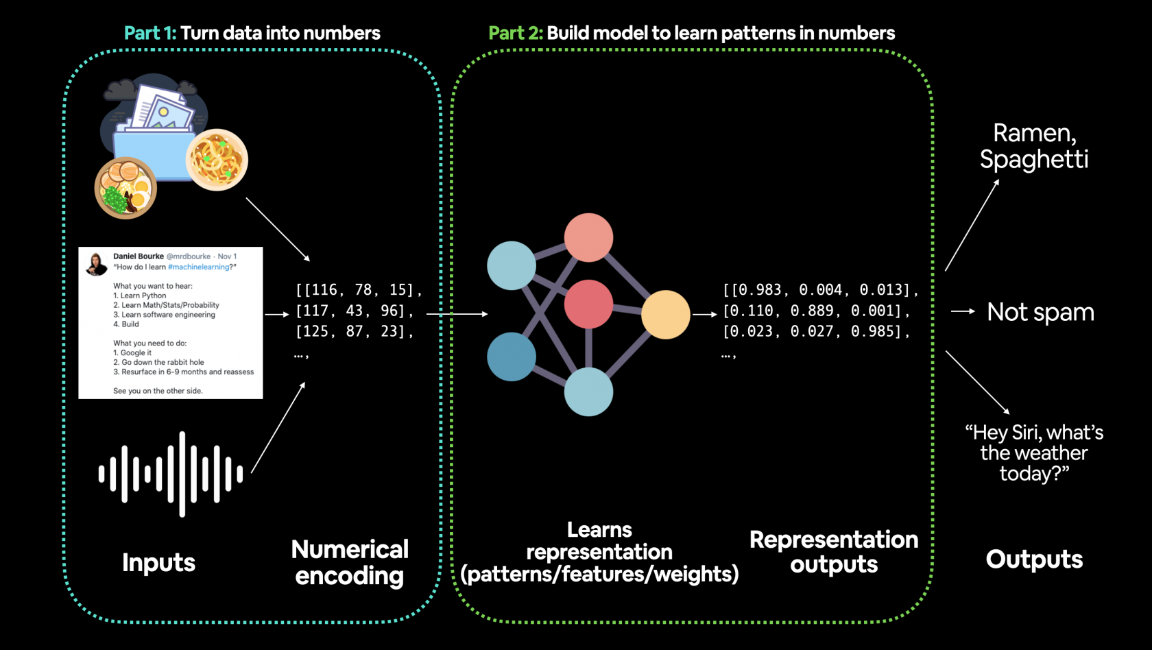
La fase iniziare e una delle più importanti nel ML è la preparazione dei dati, es:
[](https://cms.marcocucchi.it/uploads/images/gallery/2023-01/eKSPYTW36ZPG48ZQ-01-machine-learning-a-game-of-two-parts.png)
Gli step principali nella preparazione dei dati sono:
1. trasforare i dati in una rappresentazione numerica
2. costruire un modello che impari o scopra dei "pattern" nella rappresentazione numerica definita per il modello che vogliamo analizzare
Inziamo utilizzando la classica regressione lineare utilizzando la formula base y = wx + b, dove b sono i bias (detta intercetta) e w i pesi o coefficiente angolare. Per un approfondimento sulla regressione lineare vedi corso [https://cms.marcocucchi.it/books/machine-learing/page/regressione-lineare](https://cms.marcocucchi.it/books/machine-learing/page/regressione-lineare)
Ma andiamo al codice
```python
# settiamo in parametri dell'equazione
weight = 0.7
bias = 0.3
# creiamo i dati
start = 0
end = 1
step = 0.02
# agigungo una dimensione extra tramite l'unsqueeze
X = torch.arange(start, end, step).unsqueeze(dim=1)
y = weight * X + bias
X.shape, X[:10], y[:10]
>(torch.Size([50, 1]),
(tensor([[0.0000],
[0.0200],
[0.0400],
[0.0600],
[0.0800],
[0.1000],
[0.1200],
[0.1400],
[0.1600],
[0.1800]]),
tensor([[0.3000],
[0.3140],
[0.3280],
[0.3420],
[0.3560],
[0.3700],
[0.3840],
[0.3980],
[0.4120],
[0.4260]]))
```
Nell'esempio sopra riportato andremo a creare i dati relativi ad una semplice equazione lineare che verranno inviati alla rete neurale per identificare il pattern che più si avvicina all'equazione Y= vw + b che li ha originati
##### Training, Validation e Test sets
Uno dei concetti più importanti nel ML è la suddivisione dei dati in tre grupi:
| Split | Purpose | Amount of total data | How often is it used? |
|---|
| \*\*Training set\*\* | sono i dati sui quali il Pytoch si "allena" per trovare il modello | ~60-80% | Always |
| \*\*Validation set\*\* | Non sempre utilizzato, nella pratica serve per effettuare una validazione interna del training. Da notare che questi non vengono utilizzati nella fase di training, servono solo per una validazione del modello in fase di training. | ~10-20% | Often but not always |
| \*\*Testing set\*\* | Validazione finare del modello. | ~10-20% | Always |
Come splittare i dati i dati in training e testing:
```python
# Create train/test split
train_split = int(0.8 * len(X)) # 80% of data used for training set, 20% for testing
X_train, y_train = X[:train_split], y[:train_split]
X_test, y_test = X[train_split:], y[train_split:]
len(X_train), len(y_train), len(X_test), len(y_test)
```
in questo modo dividiamo i dati dove l'80% sono dedicati al training e il restante 20% per la fase di test
Visualizziamo ora i dati:
```python
def plot_predictions(train_data=X_train,
train_labels=y_train,
test_data=X_test,
test_labels=y_test,
predictions=None):
"""
Plots training data, test data and compares predictions.
"""
plt.figure(figsize=(10, 7))
# Plot training data in blue
plt.scatter(train_data, train_labels, c="b", s=4, label="Training data")
# Plot test data in green
plt.scatter(test_data, test_labels, c="g", s=4, label="Testing data")
if predictions is not None:
# Plot the predictions in red (predictions were made on the test data)
plt.scatter(test_data, predictions, c="r", s=4, label="Predictions")
# Show the legend
plt.legend(prop={"size": 14});
plot_predictions();
```
e l'output risulta:
[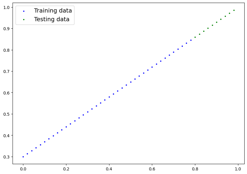](https://cms.marcocucchi.it/uploads/images/gallery/2023-01/lwHSIApmXe31WaJn-index.png)
in blu i dati di traing, mentre in verde quelli di test.
Ora creiamo il modello:
```python
# Creiamo un classe di regressione lineare che eredita da nn.Module
class LinearRegressionModel(nn.Module):
# inizializzazione delle rete neurale
def __init__(self):
super().__init__()
# normalmente le w e b sono più complesso di questo caso...
# il nome di questo tipo di variabili è arbitrario
self.weights = nn.Parameter(torch.randn(1, # generiamo un (1) tensore con un valore randomico
dtype=torch.float), # <- PyTorch preferisce utilizzare float32 by default
requires_grad=True) # pytoch aggiornerà il parametro tramite il backpropagation e discesa del gradiente
# il nome di questo tipo di variabili è arbitrario
self.bias = nn.Parameter(torch.randn(1, # generiamo un (1) tensore con un valore randomico
dtype=torch.float), # <- PyTorch preferisce utilizzare float32 by default
requires_grad=True) # pytoch aggiornerà il parametro tramite il backpropagation e discesa del gradiente
# propagazione di tipo "forward"
def forward(self, x: torch.Tensor) -> torch.Tensor: # <- "x" input data (training/testing features)
return self.weights * x + self.bias # <- questa è la formula della regressione lineare (y = m*x + b)
```
La classe torch.NN è la base per la creazione dei "grafi di neuroni", questa classe effettua due macro tipologie di operazioni, ovvero:
1. **la discesa del gradiente**
2. **la Backpropagation**
tenendo traccia della variazione dei pesi e dei bias.
Il metodo "torch.randn" può generare un tensore il cui shape è passato in input es.
```
torch.randn(2, 3)
```
##### PyTorch model building essentials
Le componenti princiali (più o meno) per creare una rete neurale in Pytorch sono:
[`torch.nn`](https://pytorch.org/docs/stable/nn.html), [`torch.optim`](https://pytorch.org/docs/stable/optim.html), [`torch.utils.data.Dataset`](https://pytorch.org/docs/stable/data.html#torch.utils.data.Dataset) and [`torch.utils.data.DataLoader`](https://pytorch.org/docs/stable/data.html). For now, we'll focus on the first two and get to the other two later (though you may be able to guess what they do).
| PyTorch module | What does it do? |
|---|
| [torch.nn](https://pytorch.org/docs/stable/nn.html) | Contains all of the building blocks for computational graphs (essentially a series of computations executed in a particular way). |
| [torch.nn.Parameter](https://pytorch.org/docs/stable/generated/torch.nn.parameter.Parameter.html#parameter) | Stores tensors that can be used with `nn.Module`. If `requires\_grad=True` gradients (used for updating model parameters via \[\*\*gradient descent\*\*\](https://ml-cheatsheet.readthedocs.io/en/latest/gradient\_descent.html)) are calculated automatically, this is often referred to as "autograd". |
| [torch.nn.Module](https://pytorch.org/docs/stable/generated/torch.nn.Module.html#torch.nn.Module) | The base class for all neural network modules, all the building blocks for neural networks are subclasses. If you're building a neural network in PyTorch, your models should subclass `nn.Module`. Requires a `forward()` method be implemented. |
| [torch.optim](https://pytorch.org/docs/stable/optim.html) | Contains various optimization algorithms (these tell the model parameters stored in `nn.Parameter` how to best change to improve gradient descent and in turn reduce the loss). |
| def forward() | All `nn.Module` subclasses require a `forward()` method, this defines the computation that will take place on the data passed to the particular `nn.Module` (e.g. the linear regression formula above). Questa classe in genere va sempre implementata
|
If the above sounds complex, think of like this, almost everything in a PyTorch neural network comes from `torch.nn`,
- `nn.Module` contains the larger building blocks (layers)
- `nn.Parameter` contains the smaller parameters like weights and biases (put these together to make `nn.Module`(s))
- `forward()` tells the larger blocks how to make calculations on inputs (tensors full of data) within `nn.Module`(s)
- `torch.optim` contains optimization methods on how to improve the parameters within `nn.Parameter` to better represent input data
[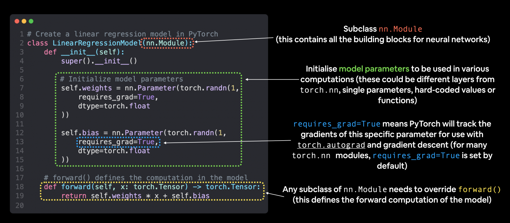](https://cms.marcocucchi.it/uploads/images/gallery/2023-01/fzZsSItdDbK57dHe-01-pytorch-linear-model-annotated.png)
Visualizziamo i valori w e b prima dell'elaboraizone:
```python
# Set manual seed since nn.Parameter are randomly initialzied
torch.manual_seed(42)
# Create an instance of the model (this is a subclass of nn.Module that contains nn.Parameter(s))
model_0 = LinearRegressionModel()
# Check the nn.Parameter(s) within the nn.Module subclass we created
list(model_0.parameters())
>[Parameter containing:
tensor([0.3367], requires_grad=True),
# vediamo la lista dei parametri
model_0.state_dict()
>OrderedDict([('weights', tensor([0.3367])), ('bias', tensor([0.1288]))])
```
proviamo a fare delle predizioni senza aver fatto il training giusto per vedere come si comporta il modello.
Per fare delle predizioni si utilizza il medoto .inference\_mode():
```python
# Make predictions with model
# con torch.inference_mode() facciamo in modo non si salvi i parametri che normalmente vengono
# utilizzati nella fase di training, cosa inutile durante la predizione in quanto il training
# dovrebbe essere già stato effettuato. In soldoni migliori performace durante la fare predittiva
with torch.inference_mode():
y_preds = model_0(X_test)
# Check the predictions
print(f"Number of testing samples: {len(X_test)}")
print(f"Number of predictions made: {len(y_preds)}")
print(f"Predicted values:\n{y_preds}")
Number of testing samples: 10
Number of predictions made: 10
Predicted values:
tensor([[0.3982],
[0.4049],
[0.4116],
[0.4184],
[0.4251],
[0.4318],
[0.4386],
[0.4453],
[0.4520],
[0.4588]])
# proviamo a visualizzare i valori della previsione
plot_predictions(predictions=y_preds)
```
[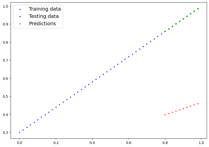](https://cms.marcocucchi.it/uploads/images/gallery/2023-01/fYUwpnvw7QlpcL6U-index.png)
e come si bene notare i valori predetti (rosso) "poco ci azzeccano" con i valori originali... quindi le predizioni sono praticamente random.
##### Training
**Loss function**
Prima di trattare il training per se vediamo di capire come misura quanto il modello si avvicina ai valori attesi o ideali, per effettuare questo controllo viene utilizzata la "loss function" o "cost function". (vedo [https://pytorch.org/docs/stable/nn.html#loss-functions](https://pytorch.org/docs/stable/nn.html#loss-functions))
Nella pratica uno dei metodi più basici è misurare la distanza tra gli attesi e i predetti.
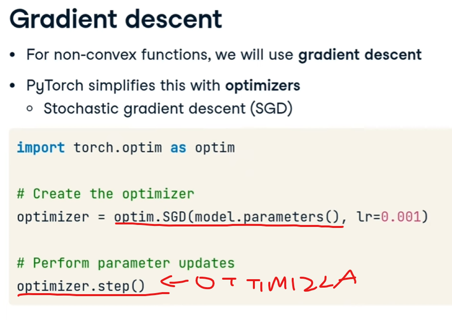
**Optimizer**
L'optimizer serve per ottimizzare i valori predetti in modo che si avvicinino sempre di più ai valori ideali, quindi per migliorare la loss function. (i cui delta vengono ritornati dalla "loss function", in modo che la loss function stessa indichi un miglioramento della predizione)
Nello specifico per pytorch servirà un training loop e un test loop.
##### Creare una loss function e un optimizer
| Function | What does it do? | Where does it live in PyTorch? | Common values |
|---|
| \*\*Loss function\*\* | Measures how wrong your models predictions (e.g. `y\_preds`) are compared to the truth labels (e.g. `y\_test`). Lower the better. vedi tabella delle loss functions:
[loss-functions](https://pytorch.org/docs/stable/nn.html#loss-functions)
| PyTorch has plenty of built-in loss functions in \[`torch.nn`\](https://pytorch.org/docs/stable/nn.html#loss-functions). | Mean absolute error (MAE) for regression problems (\[`torch.nn.L1Loss()`\](https://pytorch.org/docs/stable/generated/torch.nn.L1Loss.html)). Binary cross entropy for binary classification problems (\[`torch.nn.BCELoss()`\](https://pytorch.org/docs/stable/generated/torch.nn.BCELoss.html)). |
| \*\*Optimizer\*\* | Tells your model how to update its internal parameters to best lower the loss. vedi lista degli optimizers
[opimizers](https://pytorch.org/docs/stable/optim.html?highlight=optimizer#torch.optim.Optimizer)
| You can find various optimization function implementations in \[`torch.optim`\](https://pytorch.org/docs/stable/optim.html). | Stochastic gradient descent (\[`torch.optim.SGD()`\](https://pytorch.org/docs/stable/generated/torch.optim.SGD.html#torch.optim.SGD)). Adam optimizer (\[`torch.optim.Adam()`\](https://pytorch.org/docs/stable/generated/torch.optim.Adam.html#torch.optim.Adam)). |
Esistono varie famiglie di "**loss function**" a seconda del tipo di elaborazione, per la predizioni di valori numerici è possibile utilizzare la *Mean absolute error (MAE, in PyTorch: `torch.nn.L1Loss`)* che miura la differenze in valori assoluti tra due punti che nel nostro caso sono le "prediction" e le "label" (che sono i valori attesi) per poi calcolarne il valore medio.
Di seguito una rappresentazione grafica dello MAE, dove si evidenzia il calcolo medio della differenza in valore assoulto tra valori attesi e valori predetti.
[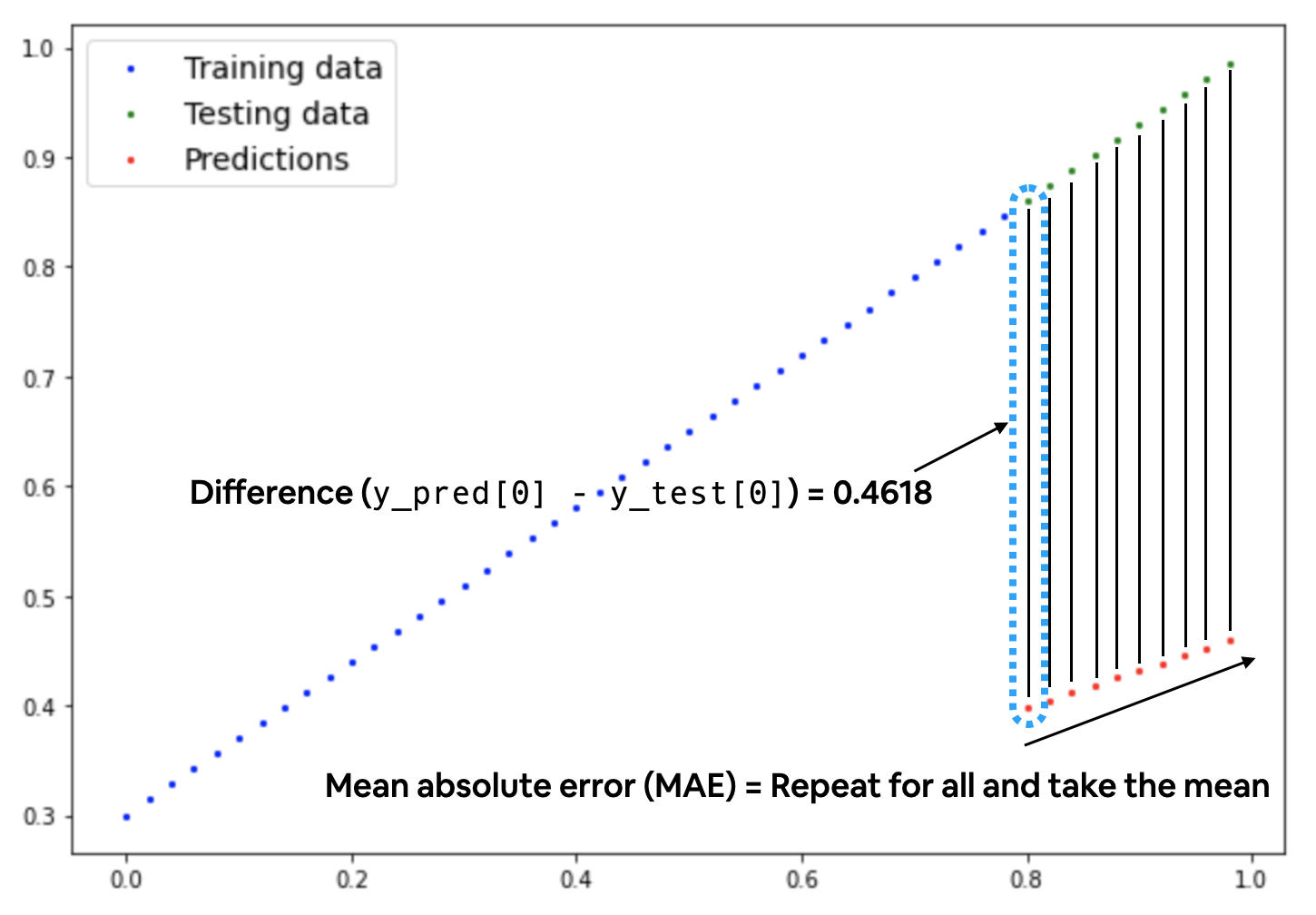](https://cms.marcocucchi.it/uploads/images/gallery/2023-01/xf6Ml7xJBjXbiRcJ-01-mae-loss-annotated.png)
quindi:
```python
# creiamo una loss function
loss_fn = nn.L1Loss() # MAE
# creiamo un optimizer, scegliamo il classico Stocastic Gradient Descent
optimizer = torch.optim.SGD(params=model_0.parameters(), # passiamo i parametri da ottimizzare (in questo caso "w" e "b"
lr=0.01) # settiamo il passo per il calcolo del gradiente, più piccolo = più tempo
```
di seguito gli step logici della fare si training:
### PyTorch training loop
For the training loop, we'll build the following steps:
| Number | Step name | What does it do? | Code example |
|---|
| 1 | Forward pass | The model goes through all of the training data once, performing its `forward()` function calculations. | *`model(x\_train)`* |
| 2 | Calculate the loss | The model's outputs (predictions) are compared to the ground truth and evaluated to see how wrong they are. | *`loss = loss\_fn(y\_pred, y\_train)`* |
| 3 | Zero gradients | The optimizers gradients are set to zero (they are accumulated by default) so they can be recalculated for the specific training step. | *`optimizer.zero\_grad()`* |
| 4 | Perform backpropagation on the loss | Computes the gradient of the loss with respect for every model parameter to be updated (each parameter with `requires\_grad=True`). This is known as \*\*backpropagation\*\*, hence "backwards". | *`loss.backward()`* |
| 5 | Update the optimizer (\*\*gradient descent\*\*) | Update the parameters with `requires\_grad=True` with respect to the loss gradients in order to improve them. | *`optimizer.step()`* |
l'algoritmo quindi si può delineare come:
[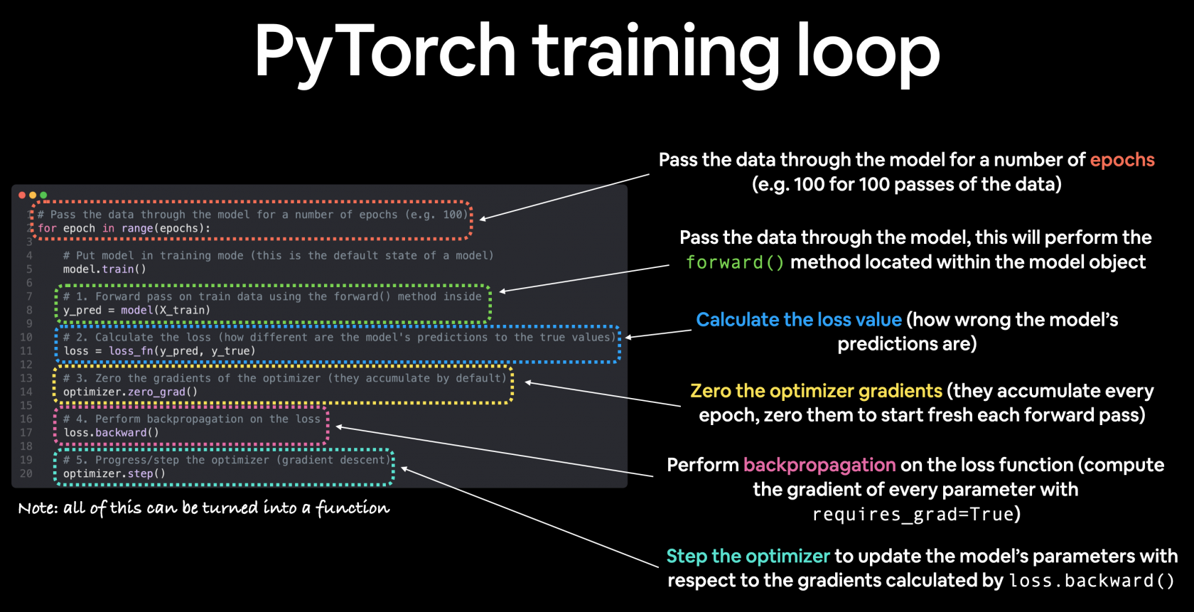](https://cms.marcocucchi.it/uploads/images/gallery/2023-01/VyAGEjCWFcQmVkpD-01-pytorch-training-loop-annotated.png)
di seguito l'algoritmo:
```python
# forzo il seed per ottenere risultati identici al
torch.manual_seed(42)
# setto le epoche, ogni epoca è un passaggio in "foward propagation" dei pesi attraverso la rete neurale
# dall'input layer all'ouout.
epochs = 100
# creo delle liste che conterranno i valori di loss per tenerne traccia durante le varie epche
train_loss_values = []
test_loss_values = []
epoch_count = []
for epoch in range(epochs):
### Training
# 0. imposto la modalità in Training (da fare ad ogni epoca)
model_0.train()
# 1. passo i dati di training al modello il quale internamente invocherè il metoto forward() definito
# quanto è stata implementata la classe che estende pytorch. Ottengo i dati che andranno poi comprati
# dalla loss per ottenerne in valore medio assoluto.
y_pred = model_0(X_train)
# print(y_pred)
# 2. calcolo la loss utilizzando la funzione definita precedentemmente.
loss = loss_fn(y_pred, y_train)
# 3. reinizializzo l'optimizer in quanto tende ad accumulare i valori
optimizer.zero_grad()
# 4. effettua la back propagation, nella pratica Pytorch tiene traccia dei valori associati alla discesa del gradiente
# Quindi calcola la derivata parziale per determinare il minimo della curva dei delta tra valori predetti e valori di test
loss.backward()
# 5. ottimizza i parametri (una sola volta) e in base al valore "lr".
# NB: cambia quindi i valori dei tensori per cercare di farli avvicinare ai valori ottimali
optimizer.step()
### Testing
# indico a Pytrch che la fase di training è terminata e che ora devo valutare i parametri e paragonarli con i valori attesi
model_0.eval()
# predico i valori in
with torch.inference_mode():
# 1. Forward pass on test data
test_pred = model_0(X_test)
# 2. Caculate loss on test data
test_loss = loss_fn(test_pred, y_test.type(torch.float)) # predictions come in torch.float datatype, so comparisons need to be done with tensors of the same type
# Print out what's happening
if epoch % 10 == 0:
epoch_count.append(epoch)
# i valori vengono convertiti in numpy in quanto sono dei tensori pytorch
train_loss_values.append(loss.numpy())
test_loss_values.append(test_loss.numpy())
print(f"Epoch: {epoch} | MAE Train Loss: {loss} | MAE Test Loss: {test_loss} ")
```
e l'output sarà:
```python
print (list(model_0.parameters()),model_0.state_dict())
Epoch: 0 | MAE Train Loss: 0.31288138031959534 | MAE Test Loss: 0.48106518387794495 delta: 0.1681838035583496
Epoch: 10 | MAE Train Loss: 0.1976713240146637 | MAE Test Loss: 0.3463551998138428 delta: 0.14868387579917908
Epoch: 20 | MAE Train Loss: 0.08908725529909134 | MAE Test Loss: 0.21729660034179688 delta: 0.12820935249328613
Epoch: 30 | MAE Train Loss: 0.053148526698350906 | MAE Test Loss: 0.14464017748832703 delta: 0.09149165451526642
Epoch: 40 | MAE Train Loss: 0.04543796554207802 | MAE Test Loss: 0.11360953003168106 delta: 0.06817156076431274
Epoch: 50 | MAE Train Loss: 0.04167863354086876 | MAE Test Loss: 0.09919948130846024 delta: 0.057520847767591476
Epoch: 60 | MAE Train Loss: 0.03818932920694351 | MAE Test Loss: 0.08886633068323135 delta: 0.05067700147628784
Epoch: 70 | MAE Train Loss: 0.03476089984178543 | MAE Test Loss: 0.0805937647819519 delta: 0.04583286494016647
Epoch: 80 | MAE Train Loss: 0.03132382780313492 | MAE Test Loss: 0.07232122868299484 delta: 0.040997400879859924
Epoch: 90 | MAE Train Loss: 0.02788739837706089 | MAE Test Loss: 0.06473556160926819 delta: 0.03684816509485245
Epoch: 100 | MAE Train Loss: 0.024458957836031914 | MAE Test Loss: 0.05646304413676262 delta: 0.032004088163375854
Epoch: 110 | MAE Train Loss: 0.021020207554101944 | MAE Test Loss: 0.04819049686193466 delta: 0.027170289307832718
Epoch: 120 | MAE Train Loss: 0.01758546568453312 | MAE Test Loss: 0.04060482233762741 delta: 0.02301935665309429
Epoch: 130 | MAE Train Loss: 0.014155393466353416 | MAE Test Loss: 0.03233227878808975 delta: 0.018176885321736336
Epoch: 140 | MAE Train Loss: 0.010716589167714119 | MAE Test Loss: 0.024059748277068138 delta: 0.01334315910935402
Epoch: 150 | MAE Train Loss: 0.0072835334576666355 | MAE Test Loss: 0.016474086791276932 delta: 0.009190553799271584
Epoch: 160 | MAE Train Loss: 0.0038517764769494534 | MAE Test Loss: 0.008201557211577892 delta: 0.004349780734628439
Epoch: 170 | MAE Train Loss: 0.008932482451200485 | MAE Test Loss: 0.005023092031478882 delta: -0.003909390419721603
Epoch: 180 | MAE Train Loss: 0.008932482451200485 | MAE Test Loss: 0.005023092031478882 delta: -0.003909390419721603
[Parameter containing:
tensor([0.6990], requires_grad=True), Parameter containing:
tensor([0.3093], requires_grad=True)] OrderedDict([('weights', tensor([0.6990])), ('bias', tensor([0.3093]))])
```
Mostriamo il grafico dei loss sul training e sui dati di testing
```python
# Plot the loss curves
plt.plot(epoch_count, train_loss_values, label="Train loss")
plt.plot(epoch_count, test_loss_values, label="Test loss")
plt.title("Training and test loss curves")
plt.ylabel("Loss")
plt.xlabel("Epochs")
plt.legend();
```
[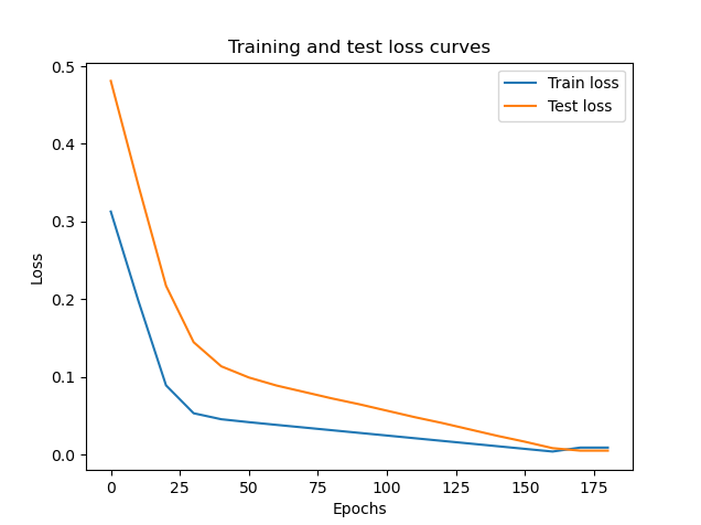](https://cms.marcocucchi.it/uploads/images/gallery/2023-01/lNMAzYCCjf0rFLQu-index.png)
e vediamo il grafico dei valori predetti vs i valori utilizzati per il traing
[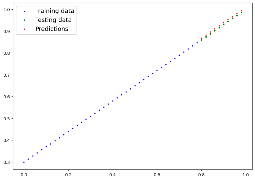](https://cms.marcocucchi.it/uploads/images/gallery/2023-01/yLbnyiosgd5nR2ZZ-index.png)
si può notare che dopo 180 epoche di training il modello riesce a predirre valori molto simili a quelli utilizzati per il training.
##### Salvare e caricare i parametri del modello
Dopo avere trovato i valori che meglio rappresentano il modello che vogliamo riprodurre vogliamo salvare i valori della rete neurale in modo da poterli ricaricare in un secondo momento senza dover riallenare la rete. Pytorch mette a disposizioni i metodo save e load per salvare su file system i parametri.
| PyTorch method | What does it do? |
|---|
| [torch.save](https://pytorch.org/docs/stable/torch.html?highlight=save#torch.save) | Saves a serialzed object to disk using Python's \[`pickle`\](https://docs.python.org/3/library/pickle.html) utility. Models, tensors and various other Python objects like dictionaries can be saved using `torch.save`. |
| [torch.load](https://pytorch.org/docs/stable/torch.html?highlight=torch%20load#torch.load)) | Uses `pickle`'s unpickling features to deserialize and load pickled Python object files (like models, tensors or dictionaries) into memory. You can also set which device to load the object to (CPU, GPU etc). |
| [torch.nn.Module.load\_state\_dict](https://pytorch.org/docs/stable/generated/torch.nn.Module.html?highlight=load_state_dict#torch.nn.Module.load_state_dict) | Loads a model's parameter dictionary (`model.state\_dict()`) using a saved `state\_dict()` object |
```python
from pathlib import Path
# 1. Create models directory
MODEL_PATH = Path("C:/Users/userxx/Desktop")
MODEL_PATH.mkdir(parents=True, exist_ok=True)
# 2. Create model save path
MODEL_NAME = "01_pytorch_workflow_model_0.pth"
MODEL_SAVE_PATH = MODEL_PATH / MODEL_NAME
# 3. Save the model state dict
print(f"Saving model to: {MODEL_SAVE_PATH}")
torch.save(obj=model_0.state_dict(), # only saving the state_dict() only saves the models learned parameters
f=MODEL_SAVE_PATH)
```
verrà quindi creato un file con i bias e i weights, per caricare il modello invce:
```python
# Instantiate a new instance of our model (this will be instantiated with random weights)
loaded_model_0 = LinearRegressionModel()
# Load the state_dict of our saved model (this will update the new instance of our model with trained weights)
loaded_model_0.load_state_dict(torch.load(f=MODEL_SAVE_PATH))
```
e provare il modello caricato:
```python
# 1. Put the loaded model into evaluation mode
loaded_model_0.eval()
# 2. Use the inference mode context manager to make predictions
with torch.inference_mode():
loaded_model_preds = loaded_model_0(X_test) # perform a forward pass on the test data with the loaded model
```
##### Evoluzione del modello/uso della GPU
Creiamo ora un modello in grado di gestire un numero significativamente maggiore di layers e nuroni configurandoli più facilmente:
```python
# Subclass nn.Module to make our model
class LinearRegressionModelV2(nn.Module):
def __init__(self):
super().__init__()
# utilizziamo un layer di quelli predefiniti da pytorch
# questa volta definiamo una semplice rete neurale fatta di un input layer e un output layer
# il modello libeare si basa sulla classica formula y = w*x + b
self.linear_layer = nn.Linear(in_features=1,
out_features=1)
# Definiamo la "forward computation" dove i valori i input "scorrono" attraverso
# la rete neurale defininta nel costruttore della classe
def forward(self, x: torch.Tensor) -> torch.Tensor:
return self.linear_layer(x)
# setto il seed per facilitare il check dei paramertri
torch.manual_seed(42)
model_1 = LinearRegressionModelV2()
print( model_1)
>LinearRegressionModelV2( (linear_layer): Linear(in_features=1, out_features=1, bias=True) )
print( model_1.state_dict())
>OrderedDict([('linear_layer.weight', tensor([[0.7645]])), ('linear_layer.bias', tensor([0.8300]))])
```
vediamo di forzare l'uso della GPU, se presente:
```python
# Setup device agnostic code
device = "cuda" if torch.cuda.is_available() else "cpu"
print(f"Using device: {device}")
> Using device: cuda
# Check model device
next(model_1.parameters()).device
>device(type='cpu')
```
si evince che di default viene la utilizzata la CPU, il nostro intente invece è utilizzare la GPU se presente e creare un sistema "agnostico" in grado di sfruttare le risorse al meglio, per cui settiamo il decice migliore:
```python
# Set model to GPU if it's availalble, otherwise it'll default to CPU
model_1.to(device) # the device variable was set above to be "cuda" if available or "cpu" if not
next(model_1.parameters()).device
# ora utilizza la GPU
>device(type='cuda', index=0)
```
ripetiamo il training con il nuovo modello:
```python
# Create loss function
loss_fn = nn.L1Loss()
# Create optimizer
optimizer = torch.optim.SGD(params=model_1.parameters(), # optimize newly created model's parameters
lr=0.01)
torch.manual_seed(42)
# Set the number of epochs
epochs = 1000
# !!!!!!!!!!!!!
# Put data on the available device
# Without this, error will happen (not all model/data on device)
# !!!!!!!!!!!!!
X_train = X_train.to(device)
X_test = X_test.to(device)
y_train = y_train.to(device)
y_test = y_test.to(device)
for epoch in range(epochs):
### Training
model_1.train() # train mode is on by default after construction
# 1. Forward pass
y_pred = model_1(X_train)
# 2. Calculate loss
loss = loss_fn(y_pred, y_train)
# 3. Zero grad optimizer
optimizer.zero_grad()
# 4. Loss backward
loss.backward()
# 5. Step the optimizer
optimizer.step()
### Testing
model_1.eval() # put the model in evaluation mode for testing (inference)
# 1. Forward pass
with torch.inference_mode():
test_pred = model_1(X_test)
# 2. Calculate the loss
test_loss = loss_fn(test_pred, y_test)
if epoch % 100 == 0:
print(f"Epoch: {epoch} | Train loss: {loss} | Test loss: {test_loss}")
```
e l'output:
```python
# Find our model's learned parameters
from pprint import pprint # pprint = pretty print, see: https://docs.python.org/3/library/pprint.html
print("The model learned the following values for weights and bias:")
pprint(model_1.state_dict())
print("\nAnd the original values for weights and bias are:")
print(f"weights: {weight}, bias: {bias}")
The model learned the following values for weights and bias:
OrderedDict([('linear_layer.weight', tensor([[0.6968]], device='cuda:0')),
('linear_layer.bias', tensor([0.3025], device='cuda:0'))])
And the original values for weights and bias are:
weights: 0.7, bias: 0.3
```
Fare delle previsioni
```python
# Turn model into evaluation mode
model_1.eval()
# Make predictions on the test data
with torch.inference_mode():
y_preds = model_1(X_test)
print(y_preds)
tensor([[0.8600],
[0.8739],
[0.8878],
[0.9018],
[0.9157],
[0.9296],
[0.9436],
[0.9575],
[0.9714],
[0.9854]], device='cuda:0')
```
Facciamo il plot ma attenzione che i tensori sono nella GPU mentre la funzione di plot lavora con la CPU (numpy), bisognerà quindi trasferire i valori in numpy primna di plottarli.
```python
plot_predictions(predictions=y_preds) # -> non funziona in quanto i dati sono nella GPU
>TypeError: can't convert cuda:0 device type tensor to numpy. Use Tensor.cpu() to copy the tensor to host memory first.
# Put data on the CPU and plot it
plot_predictions(predictions=y_preds.cpu())
```
[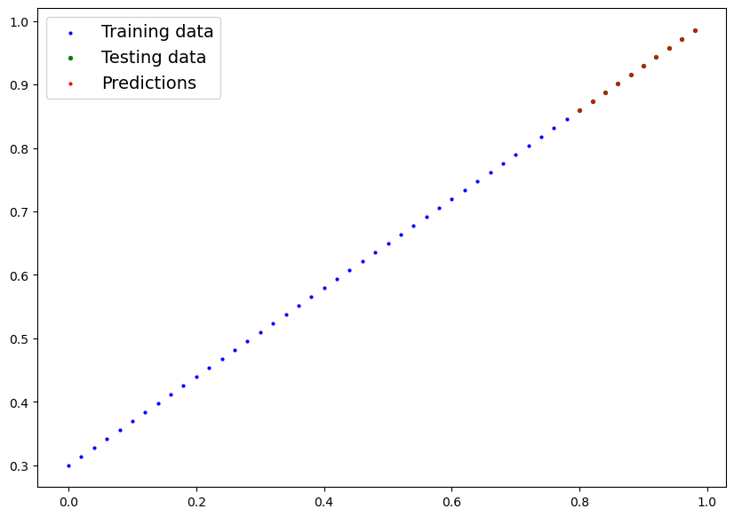](https://cms.marcocucchi.it/uploads/images/gallery/2023-01/OPH6hQ4vOY4asm2s-index.png)
##### Salvare il modello
```python
from pathlib import Path
# 1. Create models directory
MODEL_PATH = Path("path alla directoty dei modelli")
MODEL_PATH.mkdir(parents=True, exist_ok=True)
# 2. Create model save path
MODEL_NAME = "01_pytorch_workflow_model_1.pth"
MODEL_SAVE_PATH = MODEL_PATH / MODEL_NAME
# 3. Save the model state dict
print(f"Saving model to: {MODEL_SAVE_PATH}")
torch.save(obj=model_1.state_dict(), # only saving the state_dict() only saves the models learned parameters
f=MODEL_SAVE_PATH)
```
##### Caricare il modello
```python
# Instantiate a fresh instance of LinearRegressionModelV2
loaded_model_1 = LinearRegressionModelV2()
# Load model state dict
loaded_model_1.load_state_dict(torch.load(MODEL_SAVE_PATH))
# Put model to target device (if your data is on GPU, model will have to be on GPU to make predictions)
loaded_model_1.to(device)
print(f"Loaded model:\n{loaded_model_1}")
print(f"Model on device:\n{next(loaded_model_1.parameters()).device}")
```
testare il modello caricato
```python
# Evaluate loaded model
loaded_model_1.eval()
with torch.inference_mode():
loaded_model_1_preds = loaded_model_1(X_test)
y_preds == loaded_model_1_preds
>tensor([[True],
[True],
[True],
[True],
[True],
[True],
[True],
[True],
[True],
[True]], device='cuda:0')
```
# Classificazione (binary classification)
#### Introduzione
In questa lezione andremo a vedere la classificazione in base a delle tipolgie di dati, differisce quindi dalla regressione che si basa sulla predizione di un valore numero.
La classificazione può essere "binaria" es. cats vs dogs, oppure multiclass classification se abbiamo più di due tipologie da classificare.
Di seguito alcuni esempi di classificazione:
[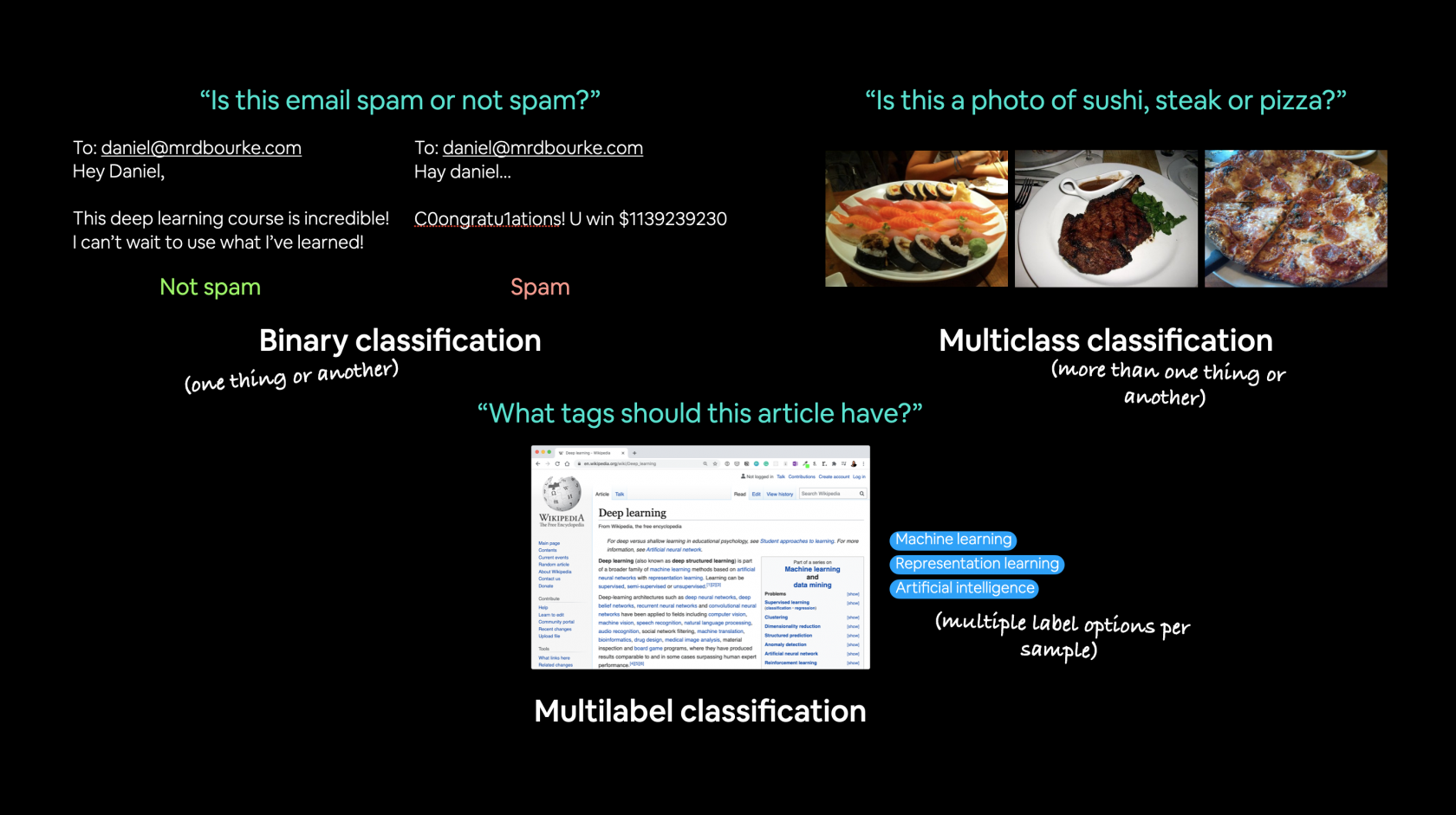](https://cms.marcocucchi.it/uploads/images/gallery/2023-01/U8lnMNeLbjbNnrEQ-02-different-classification-problems.png)
Cosa andreamo a trattare nel coso:
[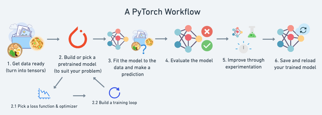](https://cms.marcocucchi.it/uploads/images/gallery/2023-01/wi3ZzDJT7iEBNtLl-01-a-pytorch-workflow.png)
| \*\*Topic\*\* | \*\*Contents\*\* |
|---|
| \*\*0. Architecture of a classification neural network\*\* | Neural networks can come in almost any shape or size, but they typically follow a similar floor plan. |
| \*\*1. Getting binary classification data ready\*\* | Data can be almost anything but to get started we're going to create a simple binary classification dataset. |
| \*\*2. Building a PyTorch classification model\*\* | Here we'll create a model to learn patterns in the data, we'll also choose a \*\*loss function\*\*, \*\*optimizer\*\* and build a \*\*training loop\*\* specific to classification. |
| \*\*3. Fitting the model to data (training)\*\* | We've got data and a model, now let's let the model (try to) find patterns in the (\*\*training\*\*) data. |
| \*\*4. Making predictions and evaluating a model (inference)\*\* | Our model's found patterns in the data, let's compare its findings to the actual (\*\*testing\*\*) data. |
| \*\*5. Improving a model (from a model perspective)\*\* | We've trained an evaluated a model but it's not working, let's try a few things to improve it. |
| \*\*6. Non-linearity\*\* | So far our model has only had the ability to model straight lines, what about non-linear (non-straight) lines? |
| \*\*7. Replicating non-linear functions\*\* | We used \*\*non-linear functions\*\* to help model non-linear data, but what do these look like? |
| \*\*8. Putting it all together with multi-class classification\*\* | Let's put everything we've done so far for binary classification together with a multi-class classification problem. |
Partiamo con un esempio di classificazione basato su due serie di cerchi che si annidano tra di loro. Utilizziamo sklearn per ottenere questo set di dati:
```python
from sklearn.datasets import make_circles
```
##### Make 1000 samples
n\_samples = 1000
```python
X, y = make_circles(n_samples,
noise=0.03, # a little bit of noise to the dots
random_state=42) # keep random state so we get the same values
```
##### Create circles
proviamo a vedere cosa contengono le X e le y.
```python
print(f"First 5 X features:\n{X[:5]}")
print(f"\nFirst 5 y labels:\n{y[:5]}")
```
First 5 X features: \[\[ 0.75424625 0.23148074\] \[-0.75615888 0.15325888\] \[-0.81539193 0.17328203\] \[-0.39373073 0.69288277\] \[ 0.44220765 -0.89672343\]\]
`First 5 y labels:[1 1 1 1 0]`
quindi le X contengono delle coordinate metre le y si suddividono in valori zero e uno. Quindi siamo di fronte ad una classificazione binaria, ma vediamola graficamente:
```python
import matplotlib.pyplot as plt
plt.scatter(x=X[:, 0],
y=X[:, 1],
c=y,
cmap=plt.cm.RdYlBu);
```
[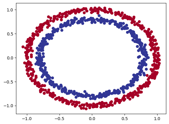](https://cms.marcocucchi.it/uploads/images/gallery/2023-01/pPZeN9JFyW8WNLG9-index.png)
Quindi riassimento le X contengo le coordinate del cerchio, mentre le y il colore. Dalla figura si vede che i cerchi sono suffidivisi in due macrogruppi posizionati uno all'interno dell'altro.
Vediamo le shape:
```python
# Check the shapes of our features and labels
X.shape, y.shape
```
`((1000, 2), (1000,))`
**X ha una shape di due, mentre le y non ha uno shape in quanto è uno scalare di un valore.**
Ora converiamo da numpy a tensori
```python
# Turn data into tensors
# Otherwise this causes issues with computations later on
import torch
X = torch.from_numpy(X).type(torch.float)
y = torch.from_numpy(y).type(torch.float)
```
#### View the first five samples
print (X\[:5\], y\[:5\])
`(tensor([[ 0.7542, 0.2315],[-0.7562, 0.1533],[-0.8154, 0.1733],[-0.3937, 0.6929],[ 0.4422, -0.8967]]),tensor([1., 1., 1., 1., 0.]))`
lo converiamo in float32 (float) perchè numpy è in float64
splittiamo i dati in training e test
```python
# Split data into train and test sets
from sklearn.model_selection import train_test_split
X_train, X_test, y_train, y_test = train_test_split(X, y, test_size=0.2, random_state=42) # make the random split
```
La funziona "**train\_test\_split**" splitta le featurues e le label per noi. :)
Bene, ora costruiamo il modello:
```python
# Standard PyTorch imports
import torch
from torch import nn
# Make device agnostic code
device = "cuda" if torch.cuda.is_available() else "cpu" device
```
#### Construct a model class that subclasses nn.Module
```python
class CircleModelV0(nn.Module):
def init(self):
super().init()
# 2. Create 2 nn.Linear layers capable of handling X and y input and output shapes
self.layer_1 = nn.Linear(in_features=2, out_features=5)
# takes in 2 features (X), produces 5 features
self.layer_2 = nn.Linear(in_features=5, out_features=1) # takes in 5 features, produces 1 feature (y)
# 3. Define a forward method containing the forward pass computation
def forward(self, x):
# Return the output of layer_2, a single feature, the same shape as y
return self.layer_2(self.layer_1(x)) # computation goes through layer_1 first then the output of layer_1 goes through layer_2
```
#### Create an instance of the model and send it to target device
`model_0 = CircleModelV0().to(device)model_0`
**NB**: una regola per settare il numero di feautres in **input** è fallo coincidere con le features del dataset. Idem per le features di **output**.
esiste inoltre un altro modo per rappresentare il modello in stile "Tensorflow", es:
```python
# costruisco il modello
model_0 = nn.Sequential(
nn.Linear(in_features=2, out_features=6),
nn.Linear(in_features=6, out_features=2),
nn.Linear(in_features=2, out_features=1)
).to(device)
```
`model_0`
Questo tipo di definizione del modello è "limitato" dal fatto che è sequenziale e quindi meno flessibile rispetto a reti più articolate.
Il modello può essere rappresentato graficamente come sotto riportato:
[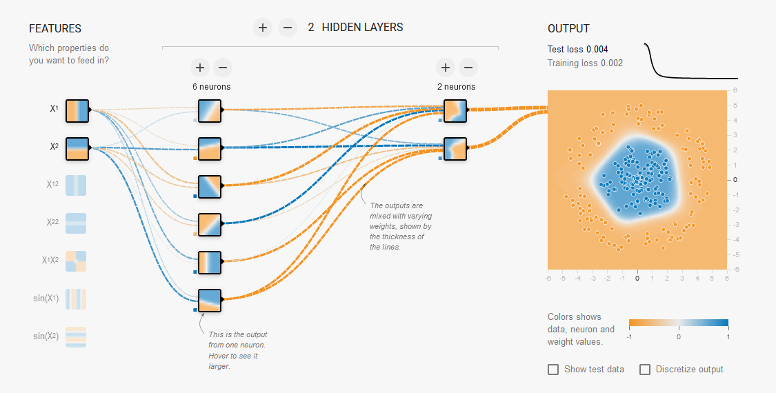](https://cms.marcocucchi.it/uploads/images/gallery/2023-01/KRZcalfDnJyr2Edj-screenshot-2023-01-14-172821.png)
[playground.tensorflow.org](https://playground.tensorflow.org)
ora, prima di fare il training del modello proviamo a passare i dati di test per vedere che output viene generato. (ovviamente essendo un modello non "allenato" saranno dati casuali)
```python
# Make predictions with the model
with torch.inference_mode():
untrained_preds = model_0(X_test.to(device))
print(f"Length of predictions: {len(untrained_preds)}, Shape: {untrained_preds.shape}")
print(f"Length of test samples: {len(y_test)}, Shape: {y_test.shape}")
print(f"\nFirst 10 predictions:\n{untrained_preds[:10]}")
print(f"\nFirst 10 test labels:\n{y_test[:10]}")
```
Length of predictions: 200, Shape: torch.Size(\[200, 1\]) Length of test samples: 200, Shape: torch.Size(\[200\])
First 10 predictions: tensor(\[\[-0.7534\], \[-0.6841\], \[-0.7949\], \[-0.7423\], \[-0.5721\], \[-0.5315\], \[-0.5128\], \[-0.4765\], \[-0.8042\], \[-0.6770\]\], device='cuda:0', grad\_fn=<SliceBackward0>)
`First 10 test labels:tensor([1., 0., 1., 0., 1., 1., 0., 0., 1., 0.])`
Possiamo notare che che l'output non è zero oppure uno come invce sono le labels... come mai? lo vedremo più avanti...
Prima di fare il training settiamo la "loss function" e "l'optimizer".
##### Setup loss function and optimizer
La domanda che ci si pone di sempre quale loss function e optimizer utilzzare?
Per la classfificazione in genere si utilizza la binary cross entropy, vedi tabella esempio sotto ripotata:
| Loss function/Optimizer | Problem type | PyTorch Code |
|---|
| Stochastic Gradient Descent (SGD) optimizer | Classification, regression, many others. | torch.optim.SGD()(https://pytorch.org/docs/stable/generated/torch.optim.SGD.html) |
| Adam Optimizer | Classification, regression, many others. | torch.optim.Adam()
`https://pytorch.org/docs/stable/generated/torch.optim.Adam.html)
|
| Binary cross entropy loss | Binary classification | torch.nn.BCELossWithLogits(
https://pytorch.org/docs/stable/generated/torch.nn.BCEWithLogitsLoss.html) or \[`torch.nn.BCELoss`\](https://pytorch.org/docs/stable/generated/torch.nn.BCELoss.html)
|
| Cross entropy loss | Mutli-class classification | \[`torch.nn.CrossEntropyLoss`\](https://pytorch.org/docs/stable/generated/torch.nn.CrossEntropyLoss.html) |
| Mean absolute error (MAE) or L1 Loss | Regression | \[`torch.nn.L1Loss`\](https://pytorch.org/docs/stable/generated/torch.nn.L1Loss.html) |
| Mean squared error (MSE) or L2 Loss | Regression | \[`torch.nn.MSELoss`\](https://pytorch.org/docs/stable/generated/torch.nn.MSELoss.html#torch.nn.MSELoss) |
Riassumento la **loss function misura** quanto il modello si distanzia dai valori attesi.
Mentre per gli **optimizer** servono per migliorare il modello che poi attraverso la loss funzion verrà valutato.
In genere si utilizza **SGD** o **Adam**..
Ok creiamo la loss e l'optimizer:
```python
# Create a loss function
# loss_fn = nn.BCELoss() # BCELoss = no sigmoid built-in
loss_fn = nn.BCEWithLogitsLoss() # BCEWithLogitsLoss = sigmoid built-in
```
##### Create an optimizer
`optimizer = torch.optim.SGD(params=model_0.parameters(), lr=0.1)`
##### Accuracy e Loss function
Definiamo anche il concetto di "**accuracy**".
La loss functuon misura quanto le preduzioni si allontanano dai valori desierati, mentre la **Accuracy** indica la **percentuale **con la quale il modello fa delle previsioni corrette. La differenza è sottile, e in questo momento non mi è chiara, credo che l'accuracy dipenda dalla loss e che indichi con una percentuale quello che la loss esprime in valori numerici specifici per il modello. Ad ogni modo vengono utilizzate entramb le misure per verificare la buona qualità del modello.
Implementiamo la accuracy
```python
# Calculate accuracy (a classification metric)
def accuracy_fn(y_true, y_pred):
correct = torch.eq(y_true, y_pred).sum().item() # torch.eq() calculates where two tensors are equal
acc = (correct / len(y_pred)) * 100
return acc
```
##### Logits
I logits rappresentano l'output "grezzo" del modello. I logits devono essere convertiti nella previsione probabilistica passandoli ad una "funzione di attivazione". (es. sigmoid per la "binari cross entropy", softmax per la multiclass classificazion) Per noi essere "discretizzati" (i valori probabilistici) mediante l'uso di funzioni come "round".
Vediamo quindi come rivedere la fase di training in funzione dei logits. NB per capire la rappresentazione dei logits vedi il commento nel training loop.
```python
for epoch in range(epochs):
### Training
# 0. imposto la modalità in Training (da fare ad ogni epoca)
model_0.train()
# 1. calcolo l'output con i parametri del modello, NB devo gare la "squeeze" percheè va ritdotta di una dimensione
# quanto l'output del modello ne aggiunge una.
# I logits sono i valori "grezzi" che, nella caso delle classificazioni BINARIE, NON possono essere comparati
# con i valori discreti 0/1 delle t_test.
# I logits quindive dobranno essere convertiti attraverso le funzioni come per la esempio la sigmoing, che
# non fa altro che ricondurli a valori compresi tra zero e uno che, poi andranno "discretizzati" a 0/1 atttraverso
# l'uso di funzioni di arrotondamento come per es. la round.
y_logits = model_0(X_train).squeeze() #
# pred. logits -> pred. probabilities -> labels 0/1
y_pred = torch.round(torch.sigmoid(y_logits))
# 2. calculate loss/accuracy
# calcolo la loss, da nota che viene utilizzata come loss function la "BCEWithLogitsLoss" che vuole in input
# dirattamente i logits anzichè i valori predetti, in quanto gli applica la sigmoid e la round in automatico
# per poi paragonli con le y_train "discrete".
loss = loss_fn(y_logits, y_train) # nn.BCEWithLogitsLoss()
# calcololiamo anche la percentuale di accuratezza.
acc = accuracy_fn(y_true=y_train, y_pred=y_pred)
# 3. reinizializzo l'optimizer in quanto tende ad accumulare i valori
optimizer.zero_grad()
# 4. effettua la back propagation, nella pratica Pytorch tiene traccia dei valori associati alla discesa del gradiente
# Quindi calcola la derivata parziale per determinare il minimo della curva dei delta tra valori predetti e valori di test
loss.backward()
# 5. ottimizza i parametri (una sola volta) e in base al valore "lr".
# NB: cambia quindi i valori dei tensori per cercare di farli avvicinare ai valori ottimali
optimizer.step()
### Testing (in questa fase vengono passati i valori non trainati di test)
# indico a Pytrch che la fase di training è terminata e che ora devo valutare i parametri e paragonarli con i valori attesi
model_0.eval()
with torch.inference_mode(): # disabilito la fase di training
test_logits = model_0(X_test).squeeze() #
# pred. logits -> pred. probabilities -> labels 0/1
test_pred = torch.round(torch.sigmoid(test_logits))
# per poi paragonli con le y_train "discrete".
test_loss = loss_fn(test_logits, y_test) # nn.BCEWithLogitsLoss()
# calcololiamo anche la percentuale di accuratezza.
test_acc = accuracy_fn(y_true=y_test, y_pred=test_pred)
# Print out what's happening
if epoch % 10 == 0:
print(f"Epoch: {epoch} | Train -> Loss: {loss:.5f} , Acc: {acc:.2f}% | Test -> Loss: {test_loss:.5f}%. Acc: {test_acc:.2f}% ")
```
L'output della funzione sarà:
```bash
Python 3.10.8 | packaged by conda-forge | (main, Nov 24 2022, 14:07:00) [MSC v.1916 64 bit (AMD64)]
Type 'copyright', 'credits' or 'license' for more information
IPython 8.7.0 -- An enhanced Interactive Python. Type '?' for help.
PyDev console: using IPython 8.7.0
Python 3.10.8 | packaged by conda-forge | (main, Nov 24 2022, 14:07:00) [MSC v.1916 64 bit (AMD64)] on win32
runfile('C:\\lavori\\formazione_py\\src\\formazione\\DanielBourkePytorch\\02_classification.py', wdir='C:\\lavori\\formazione_py\\src\\formazione\\DanielBourkePytorch')
Epoch: 0 | Train -> Loss: 0.70155 , Acc: 50.00% | Test -> Loss: 0.70146%. Acc: 50.00%
Epoch: 10 | Train -> Loss: 0.69617 , Acc: 57.50% | Test -> Loss: 0.69654%. Acc: 55.50%
Epoch: 20 | Train -> Loss: 0.69453 , Acc: 51.75% | Test -> Loss: 0.69501%. Acc: 54.50%
Epoch: 30 | Train -> Loss: 0.69395 , Acc: 50.38% | Test -> Loss: 0.69448%. Acc: 53.50%
Epoch: 40 | Train -> Loss: 0.69370 , Acc: 49.50% | Test -> Loss: 0.69427%. Acc: 53.50%
Epoch: 50 | Train -> Loss: 0.69358 , Acc: 49.50% | Test -> Loss: 0.69417%. Acc: 53.00%
Epoch: 60 | Train -> Loss: 0.69349 , Acc: 49.88% | Test -> Loss: 0.69412%. Acc: 52.00%
Epoch: 70 | Train -> Loss: 0.69343 , Acc: 49.62% | Test -> Loss: 0.69409%. Acc: 51.50%
Epoch: 80 | Train -> Loss: 0.69337 , Acc: 49.25% | Test -> Loss: 0.69408%. Acc: 51.50%
Epoch: 90 | Train -> Loss: 0.69333 , Acc: 49.62% | Test -> Loss: 0.69407%. Acc: 51.50%
Backend MacOSX is interactive backend. Turning interactive mode on.
```
che è pessimo in quanto il modello utilizza un "linear model" che sostanzialmente rappresenta una linea che negli assi cartesiani ha un'intercetta e una direzione e quindi non riscurà mai a rappresentare i dati.
[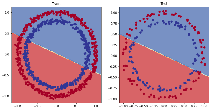](https://cms.marcocucchi.it/uploads/images/gallery/2023-05/biYPP4eEHzxwKlYC-download.png)
Bisoga quindi cambiare modello.
In particolare bisogna introdurre una funziona **non lineare** come per es. la ReLU che nella prarica ritorna zero se i valori sono <=0 oppure il valore stesso se >0.
Di seguito il grafico della funzione non lineare ReLU.
[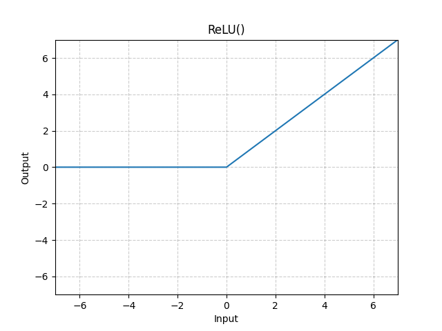](https://cms.marcocucchi.it/uploads/images/gallery/2023-05/QYo3IsNHqQ2QMxYG-relu.png)
Modifichiamo quindi il modello aggiungendo dopo l'hidden layer la funzione di attivazione non lineare come nell'esempio di seguito:
```python
# costruisco il modello
model_0 = nn.Sequential(
nn.Linear(in_features=2, out_features=10),
nn.ReLU(),
nn.Linear(in_features=10, out_features=10),
nn.ReLU(),
nn.Linear(in_features=10, out_features=1))
```
che produce risultati decisamente migliori:
Epoch: 0 | Train -> Loss: 0.69656 , Acc: 47.38% | Test -> Loss: 0.69921%. Acc: 46.00%
Epoch: 10 | Train -> Loss: 0.69417 , Acc: 46.00% | Test -> Loss: 0.69735%. Acc: 43.00%
Epoch: 20 | Train -> Loss: 0.69257 , Acc: 49.62% | Test -> Loss: 0.69603%. Acc: 49.50%
Epoch: 30 | Train -> Loss: 0.69123 , Acc: 50.38% | Test -> Loss: 0.69486%. Acc: 48.50%
Epoch: 40 | Train -> Loss: 0.69000 , Acc: 51.00% | Test -> Loss: 0.69374%. Acc: 49.50%
Epoch: 50 | Train -> Loss: 0.68884 , Acc: 51.50% | Test -> Loss: 0.69266%. Acc: 49.50%
Epoch: 60 | Train -> Loss: 0.68772 , Acc: 52.62% | Test -> Loss: 0.69162%. Acc: 48.50%
Epoch: 70 | Train -> Loss: 0.68663 , Acc: 53.00% | Test -> Loss: 0.69060%. Acc: 49.00%
Epoch: 80 | Train -> Loss: 0.68557 , Acc: 53.25% | Test -> Loss: 0.68960%. Acc: 48.50%
Epoch: 90 | Train -> Loss: 0.68453 , Acc: 53.25% | Test -> Loss: 0.68862%. Acc: 48.50%
Epoch: 100 | Train -> Loss: 0.68349 , Acc: 54.12% | Test -> Loss: 0.68765%. Acc: 49.00%
Epoch: 110 | Train -> Loss: 0.68246 , Acc: 54.37% | Test -> Loss: 0.68670%. Acc: 48.50%
Epoch: 120 | Train -> Loss: 0.68143 , Acc: 54.87% | Test -> Loss: 0.68574%. Acc: 49.00%
Epoch: 130 | Train -> Loss: 0.68039 , Acc: 54.75% | Test -> Loss: 0.68478%. Acc: 49.00%
Epoch: 140 | Train -> Loss: 0.67935 , Acc: 55.50% | Test -> Loss: 0.68382%. Acc: 50.00%
Epoch: 150 | Train -> Loss: 0.67829 , Acc: 55.62% | Test -> Loss: 0.68285%. Acc: 50.50%
Epoch: 160 | Train -> Loss: 0.67722 , Acc: 57.25% | Test -> Loss: 0.68188%. Acc: 53.50%
Epoch: 170 | Train -> Loss: 0.67614 , Acc: 59.62% | Test -> Loss: 0.68090%. Acc: 57.50%
Epoch: 180 | Train -> Loss: 0.67504 , Acc: 61.62% | Test -> Loss: 0.67991%. Acc: 59.00%
Epoch: 190 | Train -> Loss: 0.67390 , Acc: 63.75% | Test -> Loss: 0.67891%. Acc: 59.50%
Epoch: 200 | Train -> Loss: 0.67275 , Acc: 65.50% | Test -> Loss: 0.67789%. Acc: 60.50%
Epoch: 210 | Train -> Loss: 0.67156 , Acc: 66.50% | Test -> Loss: 0.67686%. Acc: 60.50%
Epoch: 220 | Train -> Loss: 0.67036 , Acc: 68.62% | Test -> Loss: 0.67580%. Acc: 63.50%
Epoch: 230 | Train -> Loss: 0.66912 , Acc: 70.75% | Test -> Loss: 0.67473%. Acc: 64.50%
Epoch: 240 | Train -> Loss: 0.66787 , Acc: 72.00% | Test -> Loss: 0.67363%. Acc: 66.00%
Epoch: 250 | Train -> Loss: 0.66658 , Acc: 73.75% | Test -> Loss: 0.67252%. Acc: 67.50%
Epoch: 260 | Train -> Loss: 0.66526 , Acc: 74.88% | Test -> Loss: 0.67139%. Acc: 69.00%
Epoch: 270 | Train -> Loss: 0.66392 , Acc: 75.75% | Test -> Loss: 0.67025%. Acc: 69.50%
Epoch: 280 | Train -> Loss: 0.66256 , Acc: 77.62% | Test -> Loss: 0.66909%. Acc: 72.00%
Epoch: 290 | Train -> Loss: 0.66118 , Acc: 78.75% | Test -> Loss: 0.66791%. Acc: 72.50%
Epoch: 300 | Train -> Loss: 0.65978 , Acc: 79.75% | Test -> Loss: 0.66672%. Acc: 75.50%
Epoch: 310 | Train -> Loss: 0.65835 , Acc: 80.75% | Test -> Loss: 0.66552%. Acc: 76.00%
Epoch: 320 | Train -> Loss: 0.65689 , Acc: 81.88% | Test -> Loss: 0.66431%. Acc: 77.00%
Epoch: 330 | Train -> Loss: 0.65540 , Acc: 82.75% | Test -> Loss: 0.66309%. Acc: 77.50%
Epoch: 340 | Train -> Loss: 0.65390 , Acc: 84.38% | Test -> Loss: 0.66183%. Acc: 78.50%
Epoch: 350 | Train -> Loss: 0.65237 , Acc: 85.12% | Test -> Loss: 0.66056%. Acc: 78.50%
Epoch: 360 | Train -> Loss: 0.65083 , Acc: 85.25% | Test -> Loss: 0.65927%. Acc: 81.00%
Epoch: 370 | Train -> Loss: 0.64925 , Acc: 85.88% | Test -> Loss: 0.65797%. Acc: 81.50%
Epoch: 380 | Train -> Loss: 0.64763 , Acc: 86.38% | Test -> Loss: 0.65664%. Acc: 83.00%
Epoch: 390 | Train -> Loss: 0.64599 , Acc: 87.00% | Test -> Loss: 0.65530%. Acc: 83.50%
Epoch: 400 | Train -> Loss: 0.64430 , Acc: 87.38% | Test -> Loss: 0.65394%. Acc: 84.50%
Epoch: 410 | Train -> Loss: 0.64258 , Acc: 88.75% | Test -> Loss: 0.65256%. Acc: 85.00%
Epoch: 420 | Train -> Loss: 0.64083 , Acc: 89.50% | Test -> Loss: 0.65115%. Acc: 86.00%
Epoch: 430 | Train -> Loss: 0.63904 , Acc: 89.62% | Test -> Loss: 0.64971%. Acc: 86.50%
Epoch: 440 | Train -> Loss: 0.63723 , Acc: 90.75% | Test -> Loss: 0.64825%. Acc: 87.00%
Epoch: 450 | Train -> Loss: 0.63540 , Acc: 91.38% | Test -> Loss: 0.64678%. Acc: 87.00%
Epoch: 460 | Train -> Loss: 0.63354 , Acc: 92.38% | Test -> Loss: 0.64529%. Acc: 87.00%
Epoch: 470 | Train -> Loss: 0.63165 , Acc: 93.00% | Test -> Loss: 0.64377%. Acc: 88.00%
Epoch: 480 | Train -> Loss: 0.62974 , Acc: 93.38% | Test -> Loss: 0.64222%. Acc: 89.00%
Epoch: 490 | Train -> Loss: 0.62780 , Acc: 93.50% | Test -> Loss: 0.64065%. Acc: 91.00%
Epoch: 500 | Train -> Loss: 0.62585 , Acc: 94.38% | Test -> Loss: 0.63905%. Acc: 91.50%
Epoch: 510 | Train -> Loss: 0.62386 , Acc: 94.75% | Test -> Loss: 0.63746%. Acc: 92.50%
Epoch: 520 | Train -> Loss: 0.62183 , Acc: 95.25% | Test -> Loss: 0.63584%. Acc: 92.50%
Epoch: 530 | Train -> Loss: 0.61979 , Acc: 95.50% | Test -> Loss: 0.63421%. Acc: 92.50%
Epoch: 540 | Train -> Loss: 0.61773 , Acc: 95.75% | Test -> Loss: 0.63255%. Acc: 92.50%
Epoch: 550 | Train -> Loss: 0.61564 , Acc: 95.62% | Test -> Loss: 0.63088%. Acc: 93.00%
Epoch: 560 | Train -> Loss: 0.61351 , Acc: 96.00% | Test -> Loss: 0.62917%. Acc: 93.50%
Epoch: 570 | Train -> Loss: 0.61136 , Acc: 96.00% | Test -> Loss: 0.62742%. Acc: 94.00%
Epoch: 580 | Train -> Loss: 0.60919 , Acc: 96.12% | Test -> Loss: 0.62565%. Acc: 94.50%
Epoch: 590 | Train -> Loss: 0.60699 , Acc: 96.00% | Test -> Loss: 0.62385%. Acc: 94.50%
Epoch: 600 | Train -> Loss: 0.60477 , Acc: 96.50% | Test -> Loss: 0.62203%. Acc: 94.50%
Epoch: 610 | Train -> Loss: 0.60253 , Acc: 96.50% | Test -> Loss: 0.62020%. Acc: 94.00%
Epoch: 620 | Train -> Loss: 0.60026 , Acc: 96.75% | Test -> Loss: 0.61833%. Acc: 94.00%
Epoch: 630 | Train -> Loss: 0.59796 , Acc: 97.00% | Test -> Loss: 0.61643%. Acc: 94.50%
Epoch: 640 | Train -> Loss: 0.59563 , Acc: 97.25% | Test -> Loss: 0.61449%. Acc: 94.50%
Epoch: 650 | Train -> Loss: 0.59327 , Acc: 97.38% | Test -> Loss: 0.61253%. Acc: 94.50%
Epoch: 660 | Train -> Loss: 0.59086 , Acc: 97.62% | Test -> Loss: 0.61053%. Acc: 94.50%
Epoch: 670 | Train -> Loss: 0.58843 , Acc: 97.62% | Test -> Loss: 0.60850%. Acc: 94.00%
Epoch: 680 | Train -> Loss: 0.58595 , Acc: 97.88% | Test -> Loss: 0.60642%. Acc: 95.00%
Epoch: 690 | Train -> Loss: 0.58343 , Acc: 97.88% | Test -> Loss: 0.60429%. Acc: 95.50%
Epoch: 700 | Train -> Loss: 0.58088 , Acc: 97.88% | Test -> Loss: 0.60211%. Acc: 95.50%
Epoch: 710 | Train -> Loss: 0.57830 , Acc: 98.00% | Test -> Loss: 0.59991%. Acc: 96.00%
Epoch: 720 | Train -> Loss: 0.57569 , Acc: 98.25% | Test -> Loss: 0.59767%. Acc: 96.50%
Epoch: 730 | Train -> Loss: 0.57305 , Acc: 98.38% | Test -> Loss: 0.59541%. Acc: 96.50%
Epoch: 740 | Train -> Loss: 0.57037 , Acc: 98.50% | Test -> Loss: 0.59309%. Acc: 96.50%
Epoch: 750 | Train -> Loss: 0.56766 , Acc: 98.50% | Test -> Loss: 0.59073%. Acc: 96.50%
Epoch: 760 | Train -> Loss: 0.56493 , Acc: 98.62% | Test -> Loss: 0.58835%. Acc: 97.00%
Epoch: 770 | Train -> Loss: 0.56216 , Acc: 98.62% | Test -> Loss: 0.58594%. Acc: 97.00%
Epoch: 780 | Train -> Loss: 0.55935 , Acc: 98.62% | Test -> Loss: 0.58352%. Acc: 97.00%
Epoch: 790 | Train -> Loss: 0.55652 , Acc: 98.88% | Test -> Loss: 0.58106%. Acc: 97.00%
Epoch: 800 | Train -> Loss: 0.55365 , Acc: 98.88% | Test -> Loss: 0.57855%. Acc: 97.00%
Epoch: 810 | Train -> Loss: 0.55075 , Acc: 98.88% | Test -> Loss: 0.57604%. Acc: 97.00%
Epoch: 820 | Train -> Loss: 0.54782 , Acc: 98.88% | Test -> Loss: 0.57351%. Acc: 97.00%
Epoch: 830 | Train -> Loss: 0.54485 , Acc: 99.00% | Test -> Loss: 0.57095%. Acc: 97.00%
Epoch: 840 | Train -> Loss: 0.54185 , Acc: 99.00% | Test -> Loss: 0.56836%. Acc: 97.00%
Epoch: 850 | Train -> Loss: 0.53884 , Acc: 99.00% | Test -> Loss: 0.56572%. Acc: 97.50%
Epoch: 860 | Train -> Loss: 0.53580 , Acc: 99.00% | Test -> Loss: 0.56307%. Acc: 97.50%
Epoch: 870 | Train -> Loss: 0.53274 , Acc: 99.00% | Test -> Loss: 0.56040%. Acc: 97.50%
Epoch: 880 | Train -> Loss: 0.52964 , Acc: 99.00% | Test -> Loss: 0.55773%. Acc: 97.50%
Epoch: 890 | Train -> Loss: 0.52652 , Acc: 99.12% | Test -> Loss: 0.55503%. Acc: 97.50%
Epoch: 900 | Train -> Loss: 0.52337 , Acc: 99.25% | Test -> Loss: 0.55228%. Acc: 97.50%
Epoch: 910 | Train -> Loss: 0.52019 , Acc: 99.25% | Test -> Loss: 0.54952%. Acc: 97.50%
Epoch: 920 | Train -> Loss: 0.51700 , Acc: 99.25% | Test -> Loss: 0.54673%. Acc: 97.00%
Epoch: 930 | Train -> Loss: 0.51378 , Acc: 99.25% | Test -> Loss: 0.54393%. Acc: 97.00%
Epoch: 940 | Train -> Loss: 0.51053 , Acc: 99.25% | Test -> Loss: 0.54110%. Acc: 97.50%
Epoch: 950 | Train -> Loss: 0.50726 , Acc: 99.25% | Test -> Loss: 0.53826%. Acc: 97.50%
Epoch: 960 | Train -> Loss: 0.50398 , Acc: 99.25% | Test -> Loss: 0.53538%. Acc: 97.50%
Epoch: 970 | Train -> Loss: 0.50067 , Acc: 99.38% | Test -> Loss: 0.53248%. Acc: 97.50%
Epoch: 980 | Train -> Loss: 0.49734 , Acc: 99.38% | Test -> Loss: 0.52956%. Acc: 98.00%
Epoch: 990 | Train -> Loss: 0.49399 , Acc: 99.38% | Test -> Loss: 0.52664%. Acc: 98.00% 3
Da notare che l'ultimo livello della rete neurale, (l'output level) è composto da tanti neuroni quante sono le classi da classificare. Ciascun neurone di output è associato ad una classe e ne rappresenta la probabilità che l'intput appartenga ad a Niesima classe.
**NB**: ricordo che i livelli sono "lineari", il che significa che corrispondono all'equazione y=x⋅WeightsT+bias il che significa bisogna aggiungere delle funzioni non lineari in grado di "spezzare" le equazioni lineari. Potremmo inserire, tra un livello lineare e l'altro una funzion non lineare come la ReLU.
Ovvimante se i dati sono nettamente separati e quindi una linea retta li può "dividere" allora potremmo evitare di inserire le funzioni di attivazione non lineare. Nell'esempio sopra visabile i 4 gruppi di "blobs" possono essere appunto separati da linee rette, il modello potrà quindi anche (opzionale) non utilizzare le ReLU non lineari.
Per le funzioni di attivazione non lienari vedi:
[Activation func](https://pytorch.org/docs/stable/nn.html#non-linear-activations-weighted-sum-nonlinearity)
##### La loss function
Per la classificazione multiclasse andiamo a vedere cosa pytorch offre nella pagina [Loss functions](https://pytorch.org/docs/stable/nn.html#non-linear-activations-weighted-sum-nonlinearity)
Per la binary classification in genere si usa la [`nn.BCEWithLogitsLoss`](https://pytorch.org/docs/stable/generated/torch.nn.BCEWithLogitsLoss.html#torch.nn.BCEWithLogitsLoss "torch.nn.BCEWithLogitsLoss") mentre per la multiclassification si usa la [`nn.CrossEntropyLoss`](https://pytorch.org/docs/stable/generated/torch.nn.CrossEntropyLoss.html#torch.nn.CrossEntropyLoss "torch.nn.CrossEntropyLoss")
TIP: Per la CrossEntropy fare attenzione al parametro "**weight** " da valorizzare nel caso i cui il numero di elementi delle classi sono diversi tra di loro, es. i gialli sono 100 metre i versi sono 20...
```python
loss_fn = nn.CrossEntropyLoss()
```
##### L'Optimizer
Come ottimizer possiamo utilizzare quelli generici come l'Adam o il pià classico SGD, vedi pagina [optimezers](https://pytorch.org/docs/stable/optim.html).
```python
optimizer = torch.optim.SGD(model_4.parameters(), lr=0.1)
```
##### Il training loop
```python
# Fit the model
torch.manual_seed(42)
# Set number of epochs
epochs = 100
# looppo..
for epoch in range(epochs):
### Training
model_4.train()
# 1. Forward pass
y_logits = model_4(X_blob_train) # model outputs raw logits
y_pred = torch.softmax(y_logits, dim=1).argmax(dim=1) # go from logits -> prediction probabilities -> prediction labels
# print(y_logits)
# 2. Calculate loss and accuracy
loss = loss_fn(y_logits, y_blob_train)
acc = accuracy_fn(y_true=y_blob_train,
y_pred=y_pred)
# 3. Optimizer zero grad
optimizer.zero_grad()
# 4. Loss backwards
loss.backward()
# 5. Optimizer step
optimizer.step()
### Testing
model_4.eval()
with torch.inference_mode():
# 1. Forward pass
test_logits = model_4(X_blob_test)
# NB: i logits vengono passati alla funzione softmax che restituisce la probabilità
# che un valore del vettori si verifichi... (un po' forzato ma spero renda l'idea)
test_pred = torch.softmax(test_logits, dim=1).argmax(dim=1)
# 2. Calculate test loss and accuracy
test_loss = loss_fn(test_logits, y_blob_test)
test_acc = accuracy_fn(y_true=y_blob_test,
y_pred=test_pred)
# Print out what's happening
if epoch % 10 == 0:
print(f"Epoch: {epoch} | Loss: {loss:.5f}, Acc: {acc:.2f}% | Test Loss: {test_loss:.5f}, Test Acc: {test_acc:.2f}%")
```
Importante capire il funzionamento della softmax alla quale verranno passati i logits. Per comprendere meglio la [softmax](https://machinelearningmastery.com/introduction-to-softmax-classifier-in-pytorch/) vedi link.
La classe completa:
```python
# Import dependencies
import torch
import matplotlib.pyplot as plt
from sklearn.datasets import make_blobs
from sklearn.model_selection import train_test_split
from torch import nn
import numpy as np
# Set the hyperparameters for data creation
NUM_CLASSES = 4
NUM_FEATURES = 2
RANDOM_SEED = 42
# 1. Create multi-class data
X_blob, y_blob = make_blobs(n_samples=1000,
n_features=NUM_FEATURES, # X features
centers=NUM_CLASSES, # y labels
cluster_std=1.5, # give the clusters a little shake up (try changing this to 1.0, the default)
random_state=RANDOM_SEED
)
# 2. Turn data into tensors
X_blob = torch.from_numpy(X_blob).type(torch.float)
y_blob = torch.from_numpy(y_blob).type(torch.LongTensor)
print(X_blob[:5], y_blob[:5])
# 3. Split into train and test sets
X_blob_train, X_blob_test, y_blob_train, y_blob_test = train_test_split(X_blob,
y_blob,
test_size=0.2,
random_state=RANDOM_SEED
)
# 4. Plot data
# plt.figure(figsize=(10, 7))
# plt.scatter(X_blob[:, 0], X_blob[:, 1], c=y_blob, cmap=plt.cm.RdYlBu);
# Calculate accuracy (a classification metric)
def accuracy_fn(y_true, y_pred):
correct = torch.eq(y_true, y_pred).sum().item() # torch.eq() calculates where two tensors are equal
acc = (correct / len(y_pred)) * 100
return acc
def plot_decision_boundary(model: torch.nn.Module, X: torch.Tensor, y: torch.Tensor):
"""Plots decision boundaries of model predicting on X in comparison to y.
Source - https://madewithml.com/courses/foundations/neural-networks/ (with modifications)
"""
# Put everything to CPU (works better with NumPy + Matplotlib)
model.to("cpu")
X, y = X.to("cpu"), y.to("cpu")
# Setup prediction boundaries and grid
x_min, x_max = X[:, 0].min() - 0.1, X[:, 0].max() + 0.1
y_min, y_max = X[:, 1].min() - 0.1, X[:, 1].max() + 0.1
xx, yy = np.meshgrid(np.linspace(x_min, x_max, 101), np.linspace(y_min, y_max, 101))
# Make features
X_to_pred_on = torch.from_numpy(np.column_stack((xx.ravel(), yy.ravel()))).float()
# Make predictions
model.eval()
with torch.inference_mode():
y_logits = model(X_to_pred_on)
# Test for multi-class or binary and adjust logits to prediction labels
if len(torch.unique(y)) > 2:
y_pred = torch.softmax(y_logits, dim=1).argmax(dim=1) # mutli-class
else:
y_pred = torch.round(torch.sigmoid(y_logits)) # binary
# Reshape preds and plot
y_pred = y_pred.reshape(xx.shape).detach().numpy()
plt.contourf(xx, yy, y_pred, cmap=plt.cm.RdYlBu, alpha=0.7)
plt.scatter(X[:, 0], X[:, 1], c=y, s=40, cmap=plt.cm.RdYlBu)
plt.xlim(xx.min(), xx.max())
plt.ylim(yy.min(), yy.max())
# creiamo il modello
class BlobModel(nn.Module): # la nn.Module è la superclasse da derivare per costruire un modello
# customizzo gli input al costruttore
def __init__(self, input_features, output_features, hidden_units=8):
"""Initializes all required hyperparameters for a multi-class classification model.
Args:
input_features (int): Number of input features to the model.
out_features (int): Number of output features of the model
(how many classes there are).
hidden_units (int): Number of hidden units between layers, default 8.
"""
super().__init__()
# definisco i layers e il numero di neuroni che li compongnono.
# NB: i layer sono lineari e quindi rispondono all'equazione y = xw+b
self.linear_layer_stack = nn.Sequential(
nn.Linear(in_features=input_features, out_features=hidden_units),
# nn.ReLU(), # <- does our dataset require non-linear layers? (try uncommenting and see if the results change)
nn.Linear(in_features=hidden_units, out_features=hidden_units),
# nn.ReLU(), # <- does our dataset require non-linear layers? (try uncommenting and see if the results change)
nn.Linear(in_features=hidden_units, out_features=output_features), # how many classes are there?
)
def forward(self, x):
return self.linear_layer_stack(x)
# Create an instance of BlobModel and send it to the target device
model_4 = BlobModel(input_features=NUM_FEATURES,
output_features=NUM_CLASSES,
hidden_units=8)
# Create loss and optimizer
loss_fn = nn.CrossEntropyLoss()
optimizer = torch.optim.SGD(model_4.parameters(),
lr=0.1) # exercise: try changing the learning rate here and seeing what happens to the model's performance
# Fit the model
torch.manual_seed(42)
# Set number of epochs
epochs = 100
# Put data to target device
for epoch in range(epochs):
### Training
model_4.train()
# 1. Forward pass
y_logits = model_4(X_blob_train) # model outputs raw logits
y_pred = torch.softmax(y_logits, dim=1).argmax(dim=1) # go from logits -> prediction probabilities -> prediction labels
# print(y_logits)
# 2. Calculate loss and accuracy
loss = loss_fn(y_logits, y_blob_train)
acc = accuracy_fn(y_true=y_blob_train,
y_pred=y_pred)
# 3. Optimizer zero grad
optimizer.zero_grad()
# 4. Loss backwards
loss.backward()
# 5. Optimizer step
optimizer.step()
### Testing
model_4.eval()
# setto l'inference il che sta a indicare che voglio testare il modello per fare delle previsioni
with torch.inference_mode():
# 1. Forward pass
test_logits = model_4(X_blob_test)
test_pred = torch.softmax(test_logits, dim=1).argmax(dim=1)
# 2. Calculate test loss and accuracy
test_loss = loss_fn(test_logits, y_blob_test)
test_acc = accuracy_fn(y_true=y_blob_test,
y_pred=test_pred)
# Print out what's happening
if epoch % 10 == 0:
print(f"Epoch: {epoch} | Loss: {loss:.5f}, Acc: {acc:.2f}% | Test Loss: {test_loss:.5f}, Test Acc: {test_acc:.2f}%")
plt.figure(figsize=(12, 6))
plt.subplot(1, 2, 1)
plt.title("Train")
plot_decision_boundary(model_4, X_blob_train, y_blob_train)
plt.subplot(1, 2, 2)
plt.title("Test")
plot_decision_boundary(model_4, X_blob_test, y_blob_test)
```
Il cui output sarà:
[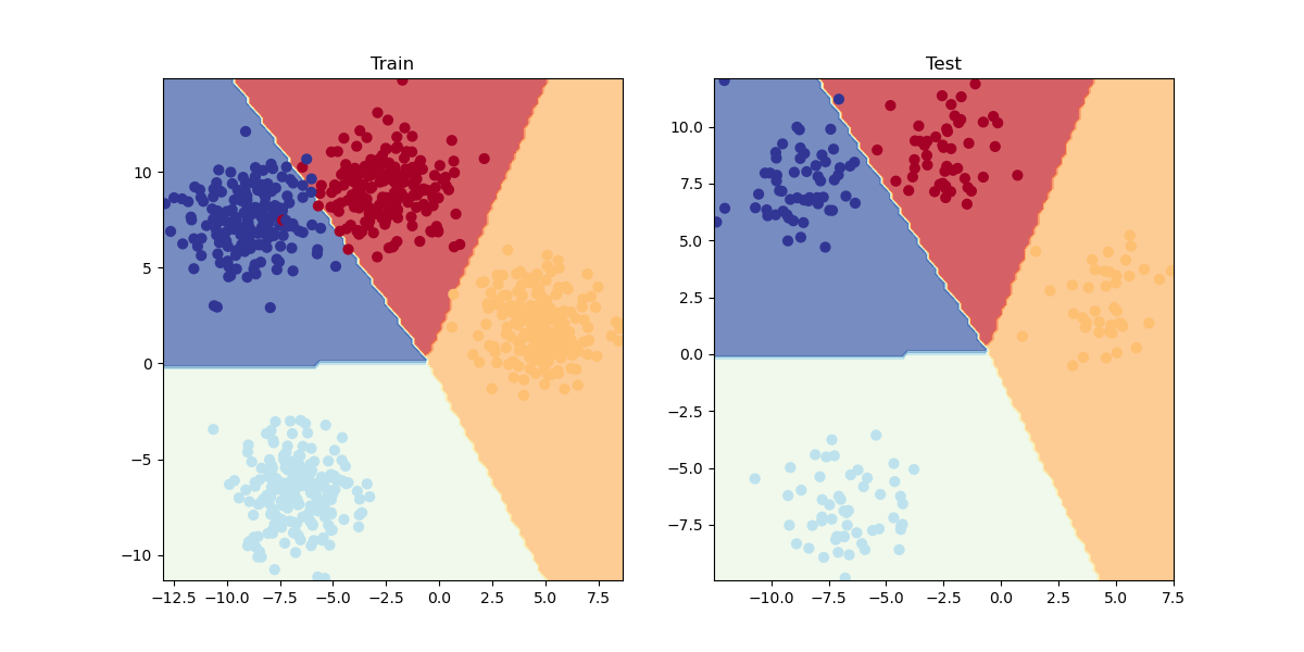](https://cms.marcocucchi.it/uploads/images/gallery/2023-05/z8VAEL4Of22W6a1s-figure-1.png)
da notare che vista la distribuzioni dei "blobs" non è necessario utilizzare funzioni non lineare come la ReLU, questo perchè i dati dei blobs sono "**separabili linearmente**", il che significa che i dati dei blobs non si michiano in maniera non lineare come per es. nel caso di due cerchi concentrici di blobs.
Il cui output è:
```bash
Python 3.10.8 | packaged by conda-forge | (main, Nov 24 2022, 14:07:00) [MSC v.1916 64 bit (AMD64)]
Type 'copyright', 'credits' or 'license' for more information
IPython 8.7.0 -- An enhanced Interactive Python. Type '?' for help.
PyDev console: using IPython 8.7.0
Python 3.10.8 | packaged by conda-forge | (main, Nov 24 2022, 14:07:00) [MSC v.1916 64 bit (AMD64)] on win32
runfile('C:\\lavori\\formazione_py\\src\\formazione\\DanielBourkePytorch\\03_multiclass_classification.py', wdir='C:\\lavori\\formazione_py\\src\\formazione\\DanielBourkePytorch')
tensor([[-8.4134, 6.9352],
[-5.7665, -6.4312],
[-6.0421, -6.7661],
[ 3.9508, 0.6984],
[ 4.2505, -0.2815]]) tensor([3, 2, 2, 1, 1])
Epoch: 0 | Loss: 1.42610, Acc: 24.12% | Test Loss: 1.14118, Test Acc: 55.00%
Epoch: 10 | Loss: 0.69430, Acc: 71.25% | Test Loss: 0.59211, Test Acc: 78.00%
Epoch: 20 | Loss: 0.54481, Acc: 72.88% | Test Loss: 0.45338, Test Acc: 79.50%
Epoch: 30 | Loss: 0.46979, Acc: 73.12% | Test Loss: 0.38420, Test Acc: 79.00%
Epoch: 40 | Loss: 0.43818, Acc: 73.12% | Test Loss: 0.35307, Test Acc: 79.00%
Epoch: 50 | Loss: 0.42259, Acc: 77.38% | Test Loss: 0.33220, Test Acc: 93.00%
Epoch: 60 | Loss: 0.12337, Acc: 99.00% | Test Loss: 0.09245, Test Acc: 99.50%
Epoch: 70 | Loss: 0.06762, Acc: 99.00% | Test Loss: 0.05245, Test Acc: 99.50%
Epoch: 80 | Loss: 0.05137, Acc: 99.00% | Test Loss: 0.03963, Test Acc: 99.50%
Epoch: 90 | Loss: 0.04380, Acc: 99.12% | Test Loss: 0.03331, Test Acc: 99.50%
Backend MacOSX is interactive backend. Turning interactive mode on.
```
# Computer vision e CNN
In questo capitolo tratteremo la computer vision e le reti convoluzionali.
In generale in Pytorch per scaricare le immagini si utilizzata la libreria "torchvision" le cui specifiche sono dettagliate nella pagina di documentazione [datasets](https://pytorch.org/vision/stable/datasets.html)
Inizieremo ad utilizzare Fashion-MNIST che contiene immagini di vestiti vedi [fashion-ds](https://github.com/zalandoresearch/fashion-mnist)
Per caricare il dataset di immagini basterà utilizzare la specifiica libreria utilizzato il metodo che ne porta il nome come sotto riportato:
```python
train_data = datasets.FashionMNIST(root='data', # dove scaricare le immagini
train=True, # si vogliono anche le immagini di training
download=True, #si vogliono scaricare
transform=torchvision.transforms.ToTensor(), # tvogliamo trasformare le immagini in tensori
target_transform=None # le immagini di test non verranno convertite in tensori
)
```
dopo aver carico le immgini di training vediamone una:
image, label = train_data[0]
e otterremo:
[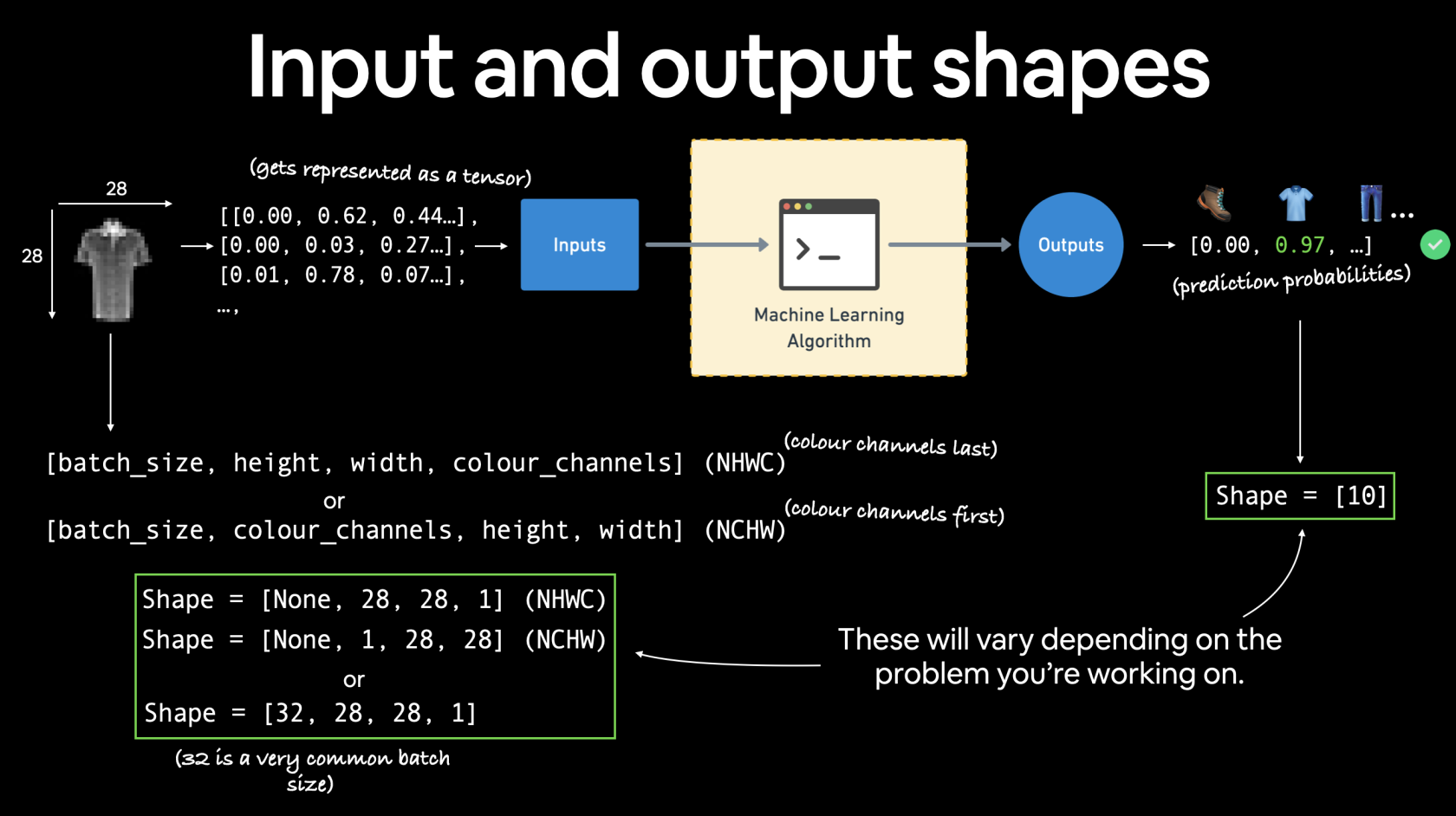](https://cms.marcocucchi.it/uploads/images/gallery/2023-05/5VcgpfIEYJBaRBMC-03-computer-vision-input-and-output-shapes.png)
Di seguito un esempio di modello lineare:
```python
@get_time
def training_model_0(device):
# creiamo il modello
class FashionMNISTModelV0(nn.Module):
def __init__(self, input_shape: int, hidden_units: int, output_shape: int):
super().__init__()
self.layer_stack = nn.Sequential(
nn.Flatten(), # neural networks like their inputs in vector form
nn.Linear(in_features=input_shape, out_features=hidden_units),
nn.ReLU(),
# in_features = number of features in a data sample (784 pixels)
nn.Linear(in_features=hidden_units, out_features=output_shape),
nn.ReLU(),
)
def forward(self, x):
return self.layer_stack(x)
# Need to setup model with input parameters
model_0 = FashionMNISTModelV0(input_shape=28 * 28, # one for every pixel (28x28)
hidden_units=10, # how many units in the hiden layer
output_shape=len(class_names) # one for every class
)
model_0.to(device) # keep model on CPU to begin with
# Setup loss function and optimizer
loss_fn = nn.CrossEntropyLoss() # this is also called "criterion"/"cost function" in some places
optimizer = torch.optim.SGD(params=model_0.parameters(), lr=0.1)
# Set the number of epochs (we'll keep this small for faster training times)
epochs = 3
# Create training and testing loop
for epoch in tqdm(range(epochs)):
print(f"Epoch: {epoch}\n-------")
### Training
train_loss = 0
# Add a loop to loop through training batches
for batch, (X, y) in enumerate(train_dataloader):
model_0.train()
y = y.to(device)
X = X.to(device)
# 1. Forward pass
y_pred = model_0(X)
# 2. Calculate loss (per batch)
loss = loss_fn(y_pred, y)
train_loss += loss # accumulatively add up the loss per epoch
# 3. Optimizer zero grad
optimizer.zero_grad()
# 4. Loss backward
loss.backward()
# 5. Optimizer step
optimizer.step()
# Print out how many samples have been seen
if batch % 400 == 0:
print(f"Looked at {batch * len(X)}/{len(train_dataloader.dataset)} samples")
# Divide total train loss by length of train dataloader (average loss per batch per epoch)
train_loss /= len(train_dataloader)
### Testing
# Setup variables for accumulatively adding up loss and accuracy
test_loss, test_acc = 0, 0
model_0.eval()
with torch.inference_mode():
for X, y in test_dataloader:
y = y.to(device)
X = X.to(device)
# 1. Forward pass
test_pred = model_0(X)
# 2. Calculate loss (accumatively)
test_loss += loss_fn(test_pred, y) # accumulatively add up the loss per epoch
# 3. Calculate accuracy (preds need to be same as y_true)
test_acc += accuracy_fn(y_true=y, y_pred=test_pred.argmax(dim=1))
# Calculations on test metrics need to happen inside torch.inference_mode()
# Divide total test loss by length of test dataloader (per batch)
test_loss /= len(test_dataloader)
# Divide total accuracy by length of test dataloader (per batch)
test_acc /= len(test_dataloader)
## Print out what's happening
print(f"\nTrain loss: {train_loss:.5f} | Test loss: {test_loss:.5f}, Test acc: {test_acc:.2f}%\n")
return model_0
```
ora, utilizzando un modello lineare non si ottengono risultati eccellenti, per la gestione della computer vision è meglio utilizzare una rete convoluzionale che fa uso per es. di layer Conv2D e MaxPool2D come sotto riportato:
[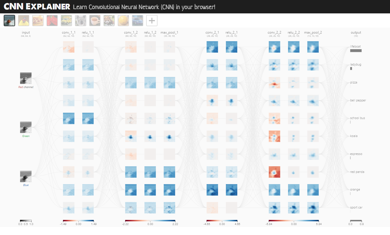](https://poloclub.github.io/cnn-explainer/)
Il layer Conv2D si occupa di trovare e evidenziare le caratteristiche più importanti dell'immagine passata in input, mediante uno scaling dell'immagine stessa applicando dei pesi a ciascun tensore che associato al pixel dell'immagine.
[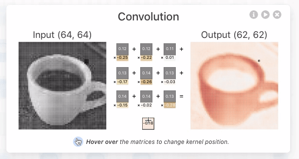](https://poloclub.github.io/cnn-explainer/ "rete convulazionale")
[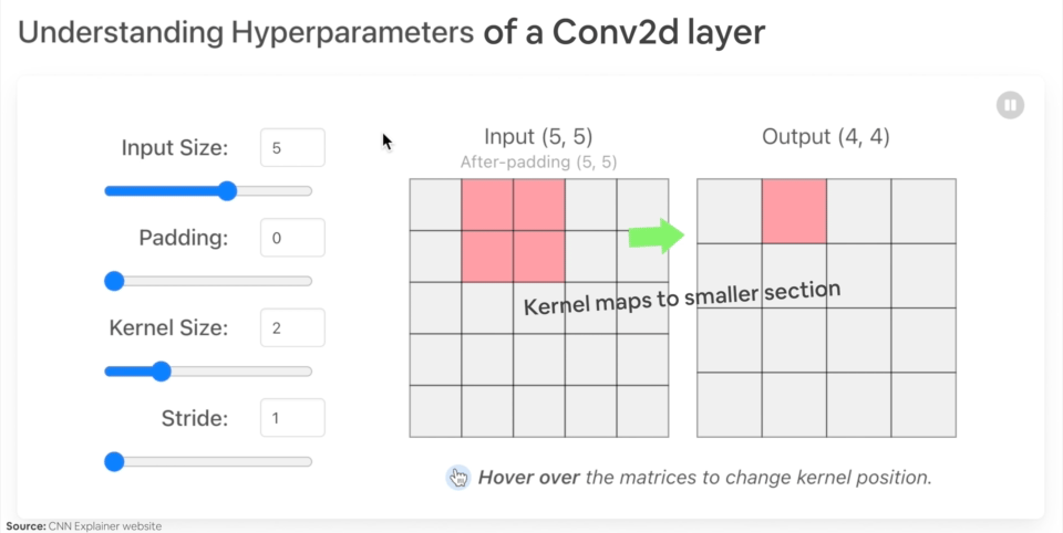](https://cms.marcocucchi.it/uploads/images/gallery/2023-06/ennEys0jJLIu7C76-image.png)
Il MaxPool2D invece scala l'imagine selezionando il tensore con valore maggiore all'interno dei un'area della matrice dei tensori.
Di seguito un esempio di rete convoluzionale in pytorch:
```python
import torch
from torch import nn
from torch.utils.data import DataLoader
import torchvision
from torchvision import datasets
from torchvision import transforms
from torchvision.transforms import ToTensor
# Import tqdm for progress bar
from tqdm.auto import tqdm
import matplotlib.pylab as plt
from src.formazione.utils.utilita import get_time
# carichiamo le immagini
train_data = datasets.FashionMNIST(root='data', # dove scaricare le immagini
train=True, # si vogliono anche le immagini di training
download=True, #si vogliono scaricare
transform=torchvision.transforms.ToTensor(), # tvogliamo trasformare le immagini in tensori
target_transform=None # le immagini di test non verranno convertite in tensori
)
test_data = datasets.FashionMNIST(root='data', # dove scaricare le immagini
train=False, # si vogliono anche le immagini di training
download=True, #si vogliono scaricare
transform=ToTensor(), # tvogliamo trasformare le immagini in tensori
target_transform=None # le immagini di test non verranno convertite in tensori
)
# nomi dei tipi di vestiti
class_names = train_data.classes
# Setup the batch size hyperparameter
BATCH_SIZE = 32
# Turn datasets into iterables (batches)
train_dataloader = DataLoader(train_data, # dataset to turn into iterable
batch_size=BATCH_SIZE, # how many samples per batch?
# num_workers =10,
shuffle=True # shuffle data every epoch?
)
test_dataloader = DataLoader(test_data,
batch_size=BATCH_SIZE,
shuffle=False # don't necessarily have to shuffle the testing data
)
def accuracy_fn(y_true, y_pred):
correct = torch.eq(y_true, y_pred).sum().item() # torch.eq() calculates where two tensors are equal
acc = (correct / len(y_pred)) * 100
return acc
# Set the seed and start the timer
torch.manual_seed(42)
@get_time
def training_model_0(device):
# creiamo il modello
class FashionMNISTModelV0(nn.Module):
def __init__(self, input_shape: int, hidden_units: int, output_shape: int):
super().__init__()
self.layer_stack = nn.Sequential(
nn.Flatten(), # neural networks like their inputs in vector form
nn.Linear(in_features=input_shape, out_features=hidden_units),
nn.ReLU(),
# in_features = number of features in a data sample (784 pixels)
nn.Linear(in_features=hidden_units, out_features=output_shape),
nn.ReLU(),
)
def forward(self, x):
return self.layer_stack(x)
# Need to setup model with input parameters
model_0 = FashionMNISTModelV0(input_shape=28 * 28, # one for every pixel (28x28)
hidden_units=10, # how many units in the hiden layer
output_shape=len(class_names) # one for every class
)
model_0.to(device) # keep model on CPU to begin with
# Setup loss function and optimizer
loss_fn = nn.CrossEntropyLoss() # this is also called "criterion"/"cost function" in some places
optimizer = torch.optim.SGD(params=model_0.parameters(), lr=0.1)
# Set the number of epochs (we'll keep this small for faster training times)
epochs = 3
# Create training and testing loop
for epoch in tqdm(range(epochs)):
print(f"Epoch: {epoch}\n-------")
### Training
train_loss = 0
# Add a loop to loop through training batches
for batch, (X, y) in enumerate(train_dataloader):
model_0.train()
y = y.to(device)
X = X.to(device)
# 1. Forward pass
y_pred = model_0(X)
# 2. Calculate loss (per batch)
loss = loss_fn(y_pred, y)
train_loss += loss # accumulatively add up the loss per epoch
# 3. Optimizer zero grad
optimizer.zero_grad()
# 4. Loss backward
loss.backward()
# 5. Optimizer step
optimizer.step()
# Print out how many samples have been seen
# if batch % 400 == 0:
# print(f"Looked at {batch * len(X)}/{len(train_dataloader.dataset)} samples")
# Divide total train loss by length of train dataloader (average loss per batch per epoch)
train_loss /= len(train_dataloader)
### Testing
# Setup variables for accumulatively adding up loss and accuracy
test_loss, test_acc = 0, 0
model_0.eval()
with torch.inference_mode():
for X, y in test_dataloader:
y = y.to(device)
X = X.to(device)
# 1. Forward pass
test_pred = model_0(X)
# 2. Calculate loss (accumatively)
test_loss += loss_fn(test_pred, y) # accumulatively add up the loss per epoch
# 3. Calculate accuracy (preds need to be same as y_true)
test_acc += accuracy_fn(y_true=y, y_pred=test_pred.argmax(dim=1))
# Calculations on test metrics need to happen inside torch.inference_mode()
# Divide total test loss by length of test dataloader (per batch)
test_loss /= len(test_dataloader)
# Divide total accuracy by length of test dataloader (per batch)
test_acc /= len(test_dataloader)
## Print out what's happening
print(f"\nTrain loss: {train_loss:.5f} | Test loss: {test_loss:.5f}, Test acc: {test_acc:.2f}%\n")
return model_0
@get_time
def training_model_2(device, epochs):
# creiamo il modello
class FashionMNISTModelV2(nn.Module):
"""
Questo modello utilizza una rete convuluzionale
"""
def __init__(self, input_shape: int, hidden_units: int, output_shape: int):
super().__init__()
padding = 1
self.con_block1 = nn.Sequential(
nn.Conv2d(in_channels=input_shape,out_channels=hidden_units, kernel_size=3, stride=1, padding=padding),
nn.ReLU(),
nn.Conv2d(in_channels=hidden_units, out_channels=hidden_units, kernel_size=3, stride=1, padding=padding),
nn.ReLU(),
nn.MaxPool2d(kernel_size=2) # prende il valore massimo dell'input portandolo in output, in pratica comprime l'input
)
self.con_block2 = nn.Sequential(
nn.Conv2d(in_channels=hidden_units ,out_channels=hidden_units, kernel_size=3, stride=1, padding=padding),
nn.ReLU(),
nn.Conv2d(in_channels=hidden_units, out_channels=hidden_units, kernel_size=3, stride=1, padding=padding),
nn.ReLU(),
nn.MaxPool2d(kernel_size=2) # prende il valore massimo dell'input portandolo in output, in pratica comprime l'input
)
self.classifier = nn.Sequential(
nn.Flatten(), # neural networks like their inputs in vector form
nn.Linear(in_features=hidden_units*7*7, out_features=hidden_units), # trucco per definire il numero di input features dopo un flatten è quello di visuallizare l'output del layer precedente
# in_features = number of features in a data sample (784 pixels)
nn.ReLU(),
nn.Linear(in_features=hidden_units, out_features=output_shape),
)
def forward(self, x):
x = self.con_block1(x)
# print(x.shape)
x = self.con_block2(x)
# print(x.shape)
x = self.classifier(x)
return x
# Need to setup model with input parameters
model_2 = FashionMNISTModelV2(
input_shape=1,
hidden_units=10, # how many units in the hiden layer
output_shape=len(class_names) # one for every class
)
model_2.to(device) # keep model on CPU to begin with
# Setup loss function and optimizer
loss_fn = nn.CrossEntropyLoss() # this is also called "criterion"/"cost function" in some places
optimizer = torch.optim.SGD(params=model_2.parameters(), lr=0.1)
# Create training and testing loop
for epoch in tqdm(range(epochs)):
# print(f"Epoch: {epoch}\n-------")
### Training
train_loss = 0
# Add a loop to loop through training batches
for batch, (X, y) in enumerate(train_dataloader):
model_2.train()
y = y.to(device)
X = X.to(device)
# 1. Forward pass
y_pred = model_2(X)
# 2. Calculate loss (per batch)
loss = loss_fn(y_pred, y)
train_loss += loss # accumulatively add up the loss per epoch
# 3. Optimizer zero grad
optimizer.zero_grad()
# 4. Loss backward
loss.backward()
# 5. Optimizer step
optimizer.step()
# Print out how many samples have been seen
# if batch % 400 == 0:
# print(f"Looked at {batch * len(X)}/{len(train_dataloader.dataset)} samples")
# Divide total train loss by length of train dataloader (average loss per batch per epoch)
train_loss /= len(train_dataloader)
### Testing
# Setup variables for accumulatively adding up loss and accuracy
test_loss, test_acc = 0, 0
model_2.eval()
with torch.inference_mode():
for X, y in test_dataloader:
y = y.to(device)
X = X.to(device)
# 1. Forward pass
test_pred = model_2(X)
# 2. Calculate loss (accumatively)
test_loss += loss_fn(test_pred, y) # accumulatively add up the loss per epoch
# 3. Calculate accuracy (preds need to be same as y_true)
test_acc += accuracy_fn(y_true=y, y_pred=test_pred.argmax(dim=1))
# Calculations on test metrics need to happen inside torch.inference_mode()
# Divide total test loss by length of test dataloader (per batch)
test_loss /= len(test_dataloader)
# Divide total accuracy by length of test dataloader (per batch)
test_acc /= len(test_dataloader)
## Print out what's happening
print(f"\nEpoch {epoch} Train loss: {train_loss:.5f} | Test loss: {test_loss:.5f}, Test acc: {test_acc:.2f}%\n")
return model_2
if __name__ == '__main__':
# training_model_0("cuda")
training_model_2("cuda", epochs=20)
```
Confusion Matrix
```python
from torchmetrics import ConfusionMatrix
from mlxtend.plotting import plot_confusion_matrix
# 2. Setup confusion matrix instance and compare predictions to targets
confmat = ConfusionMatrix(num_classes=len(class_names), task='multiclass')
confmat_tensor = confmat(preds=y_pred_tensor,
target=test_data.targets)
# 3. Plot the confusion matrix
fig, ax = plot_confusion_matrix(
conf_mat=confmat_tensor.numpy(), # matplotlib likes working with NumPy
class_names=class_names, # turn the row and column labels into class names
figsize=(10, 7)
);
```
[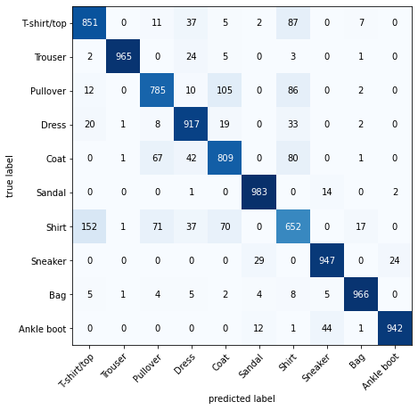](https://cms.marcocucchi.it/uploads/images/gallery/2023-06/x510sJWDunFBhbIc-image.png)
# Custom datasets
# 04. PyTorch Custom Datasets
In the last notebook, [notebook 03](https://www.learnpytorch.io/03_pytorch_computer_vision/), we looked at how to build computer vision models on an in-built dataset in PyTorch (FashionMNIST).
The steps we took are similar across many different problems in machine learning.
Find a dataset, turn the dataset into numbers, build a model (or find an existing model) to find patterns in those numbers that can be used for prediction.
PyTorch has many built-in datasets used for a wide number of machine learning benchmarks, however, you'll often want to use your own **custom dataset**.
## What is a custom dataset?
A **custom dataset** is a collection of data relating to a specific problem you're working on.
In essence, a **custom dataset** can be comprised of almost anything.
For example, if we were building a food image classification app like [Nutrify](https://nutrify.app/), our custom dataset might be images of food.
Or if we were trying to build a model to classify whether or not a text-based review on a website was positive or negative, our custom dataset might be examples of existing customer reviews and their ratings.
Or if we were trying to build a sound classification app, our custom dataset might be sound samples alongside their sample labels.
Or if we were trying to build a recommendation system for customers purchasing things on our website, our custom dataset might be examples of products other people have bought.
*PyTorch includes many existing functions to load in various custom datasets in the [`TorchVision`](https://pytorch.org/vision/stable/index.html), [`TorchText`](https://pytorch.org/text/stable/index.html), [`TorchAudio`](https://pytorch.org/audio/stable/index.html) and [`TorchRec`](https://pytorch.org/torchrec/) domain libraries.*
But sometimes these existing functions may not be enough.
In that case, we can always subclass `torch.utils.data.Dataset` and customize it to our liking.
## What we're going to cover
We're going to be applying the PyTorch Workflow we covered in [notebook 01](https://www.learnpytorch.io/01_pytorch_workflow/) and [notebook 02](https://www.learnpytorch.io/02_pytorch_classification/) to a computer vision problem.
But instead of using an in-built PyTorch dataset, we're going to be using our own dataset of pizza, steak and sushi images.
The goal will be to load these images and then build a model to train and predict on them.
*What we're going to build. We'll use `torchvision.datasets` as well as our own custom `Dataset` class to load in images of food and then we'll build a PyTorch computer vision model to hopefully be able to classify them.*
Specifically, we're going to cover:
## Where can can you get help?
All of the materials for this course [live on GitHub](https://github.com/mrdbourke/pytorch-deep-learning).
If you run into trouble, you can ask a question on the course [GitHub Discussions page](https://github.com/mrdbourke/pytorch-deep-learning/discussions) there too.
And of course, there's the [PyTorch documentation](https://pytorch.org/docs/stable/index.html) and [PyTorch developer forums](https://discuss.pytorch.org/), a very helpful place for all things PyTorch.
## 0. Importing PyTorch and setting up device-agnostic code
```
import torch
from torch import nn
# Note: this notebook requires torch >= 1.10.0
torch.__version__
```
```
'1.12.1+cu113'
```
And now let's follow best practice and setup device-agnostic code.
> **Note:** If you're using Google Colab, and you don't have a GPU turned on yet, it's now time to turn one on via `Runtime -> Change runtime type -> Hardware accelerator -> GPU`. If you do this, your runtime will likely reset and you'll have to run all of the cells above by going `Runtime -> Run before`.
```
# Setup device-agnostic code
device = "cuda" if torch.cuda.is_available() else "cpu"
device
```
```
'cuda'
```
## 1. Get data
First thing's first we need some data.
And like any good cooking show, some data has already been prepared for us.
We're going to start small.
Because we're not looking to train the biggest model or use the biggest dataset yet.
Machine learning is an iterative process, start small, get something working and increase when necessary.
The data we're going to be using is a subset of the [Food101 dataset](https://data.vision.ee.ethz.ch/cvl/datasets_extra/food-101/).
Food101 is popular computer vision benchmark as it contains 1000 images of 101 different kinds of foods, totaling 101,000 images (75,750 train and 25,250 test).
Can you think of 101 different foods?
Can you think of a computer program to classify 101 foods?
I can.
A machine learning model!
Specifically, a PyTorch computer vision model like we covered in [notebook 03](https://www.learnpytorch.io/03_pytorch_computer_vision/).
Instead of 101 food classes though, we're going to start with 3: pizza, steak and sushi.
And instead of 1,000 images per class, we're going to start with a random 10% (start small, increase when necessary).
If you'd like to see where the data came from you see the following resources:
Let's write some code to download the formatted data from GitHub.
> **Note:** The dataset we're about to use has been pre-formatted for what we'd like to use it for. However, you'll often have to format your own datasets for whatever problem you're working on. This is a regular practice in the machine learning world.
```
import requests
import zipfile
from pathlib import Path
# Setup path to data folder
data_path = Path("data/")
image_path = data_path / "pizza_steak_sushi"
# If the image folder doesn't exist, download it and prepare it...
if image_path.is_dir():
print(f"{image_path} directory exists.")
else:
print(f"Did not find {image_path} directory, creating one...")
image_path.mkdir(parents=True, exist_ok=True)
# Download pizza, steak, sushi data
with open(data_path / "pizza_steak_sushi.zip", "wb") as f:
request = requests.get("https://github.com/mrdbourke/pytorch-deep-learning/raw/main/data/pizza_steak_sushi.zip")
print("Downloading pizza, steak, sushi data...")
f.write(request.content)
# Unzip pizza, steak, sushi data
with zipfile.ZipFile(data_path / "pizza_steak_sushi.zip", "r") as zip_ref:
print("Unzipping pizza, steak, sushi data...")
zip_ref.extractall(image_path)
```
```
data/pizza_steak_sushi directory exists.
```
## 2. Become one with the data (data preparation)
Dataset downloaded!
Time to become one with it.
This is another important step before building a model.
As Abraham Lossfunction said...
*Data preparation is paramount. Before building a model, become one with the data. Ask: What am I trying to do here? Source: [@mrdbourke Twitter](https://twitter.com/mrdbourke).*
What's inspecting the data and becoming one with it?
Before starting a project or building any kind of model, it's important to know what data you're working with.
In our case, we have images of pizza, steak and sushi in standard image classification format.
Image classification format contains separate classes of images in seperate directories titled with a particular class name.
For example, all images of `pizza` are contained in the `pizza/` directory.
This format is popular across many different image classification benchmarks, including [ImageNet](https://www.image-net.org/) (of the most popular computer vision benchmark datasets).
You can see an example of the storage format below, the images numbers are arbitrary.
```
pizza_steak_sushi/ <- overall dataset folder
train/ <- training images
pizza/ <- class name as folder name
image01.jpeg
image02.jpeg
...
steak/
image24.jpeg
image25.jpeg
...
sushi/
image37.jpeg
...
test/ <- testing images
pizza/
image101.jpeg
image102.jpeg
...
steak/
image154.jpeg
image155.jpeg
...
sushi/
image167.jpeg
...
```
The goal will be to **take this data storage structure and turn it into a dataset usable with PyTorch**.
> **Note:** The structure of the data you work with will vary depending on the problem you're working on. But the premise still remains: become one with the data, then find a way to best turn it into a dataset compatible with PyTorch.
We can inspect what's in our data directory by writing a small helper function to walk through each of the subdirectories and count the files present.
To do so, we'll use Python's in-built [`os.walk()`](https://docs.python.org/3/library/os.html#os.walk).
```
import os
def walk_through_dir(dir_path):
"""
Walks through dir_path returning its contents.
Args:
dir_path (str or pathlib.Path): target directory
Returns:
A print out of:
number of subdiretories in dir_path
number of images (files) in each subdirectory
name of each subdirectory
"""
for dirpath, dirnames, filenames in os.walk(dir_path):
print(f"There are {len(dirnames)} directories and {len(filenames)} images in '{dirpath}'.")
```
```
walk_through_dir(image_path)
```
```
There are 2 directories and 1 images in 'data/pizza_steak_sushi'.
There are 3 directories and 0 images in 'data/pizza_steak_sushi/test'.
There are 0 directories and 19 images in 'data/pizza_steak_sushi/test/steak'.
There are 0 directories and 31 images in 'data/pizza_steak_sushi/test/sushi'.
There are 0 directories and 25 images in 'data/pizza_steak_sushi/test/pizza'.
There are 3 directories and 0 images in 'data/pizza_steak_sushi/train'.
There are 0 directories and 75 images in 'data/pizza_steak_sushi/train/steak'.
There are 0 directories and 72 images in 'data/pizza_steak_sushi/train/sushi'.
There are 0 directories and 78 images in 'data/pizza_steak_sushi/train/pizza'.
```
Excellent!
It looks like we've got about 75 images per training class and 25 images per testing class.
That should be enough to get started.
Remember, these images are subsets of the original Food101 dataset.
You can see how they were created in the [data creation notebook](https://github.com/mrdbourke/pytorch-deep-learning/blob/main/extras/04_custom_data_creation.ipynb).
While we're at it, let's setup our training and testing paths.
```
# Setup train and testing paths
train_dir = image_path / "train"
test_dir = image_path / "test"
train_dir, test_dir
```
```
(PosixPath('data/pizza_steak_sushi/train'),
PosixPath('data/pizza_steak_sushi/test'))
```
### 2.1 Visualize an image
Okay, we've seen how our directory structure is formatted.
Now in the spirit of the data explorer, it's time to *visualize, visualize, visualize!*
Let's write some code to:
```
import random
from PIL import Image
# Set seed
random.seed(42) # <- try changing this and see what happens
# 1. Get all image paths (* means "any combination")
image_path_list = list(image_path.glob("*/*/*.jpg"))
# 2. Get random image path
random_image_path = random.choice(image_path_list)
# 3. Get image class from path name (the image class is the name of the directory where the image is stored)
image_class = random_image_path.parent.stem
# 4. Open image
img = Image.open(random_image_path)
# 5. Print metadata
print(f"Random image path: {random_image_path}")
print(f"Image class: {image_class}")
print(f"Image height: {img.height}")
print(f"Image width: {img.width}")
img
```
```
Random image path: data/pizza_steak_sushi/test/pizza/2124579.jpg
Image class: pizza
Image height: 384
Image width: 512
```
Out[7]:

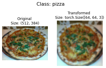
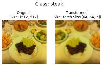
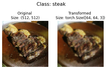
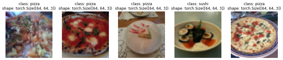
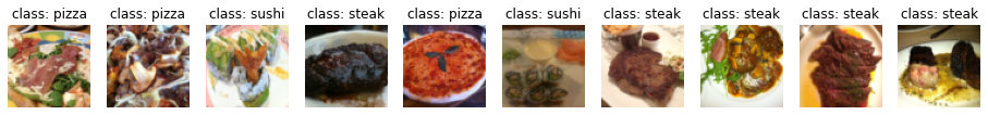
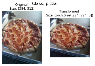
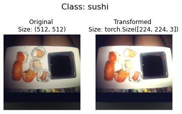
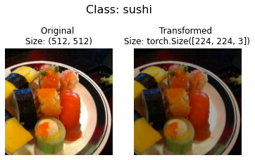
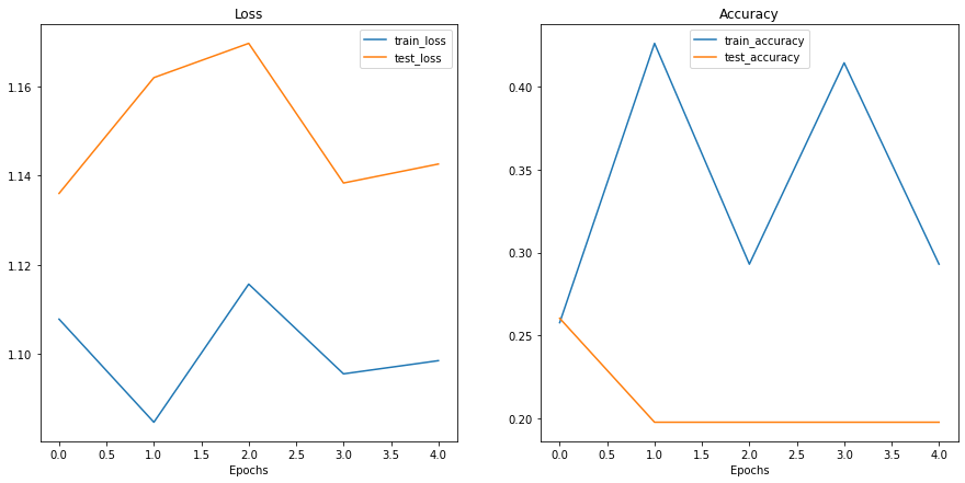
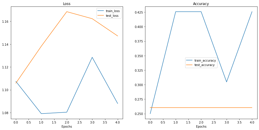
Out[57]:
| | train\_loss | train\_acc | test\_loss | test\_acc |
|---|
| 0 | 1.107833 | 0.257812 | 1.136041 | 0.260417 |
|---|
| 1 | 1.084713 | 0.425781 | 1.162014 | 0.197917 |
|---|
| 2 | 1.115697 | 0.292969 | 1.169704 | 0.197917 |
|---|
| 3 | 1.095564 | 0.414062 | 1.138373 | 0.197917 |
|---|
| 4 | 1.098520 | 0.292969 | 1.142631 | 0.197917 |
|---|
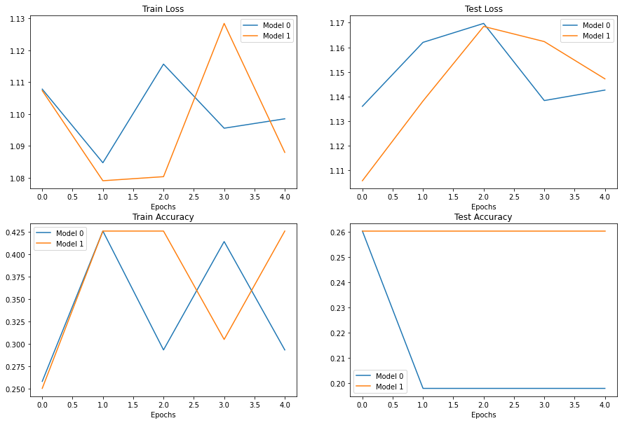
()
2 model_1.eval()
3 with torch.inference_mode():
----> 4 model_1(custom_image_uint8.to(device))
File ~/code/pytorch/env/lib/python3.8/site-packages/torch/nn/modules/module.py:1130, in Module._call_impl(self, *input, **kwargs)
1126 # If we don't have any hooks, we want to skip the rest of the logic in
1127 # this function, and just call forward.
1128 if not (self._backward_hooks or self._forward_hooks or self._forward_pre_hooks or _global_backward_hooks
1129 or _global_forward_hooks or _global_forward_pre_hooks):
-> 1130 return forward_call(*input, **kwargs)
1131 # Do not call functions when jit is used
1132 full_backward_hooks, non_full_backward_hooks = [], []
Input In [41], in TinyVGG.forward(self, x)
39 def forward(self, x: torch.Tensor):
---> 40 x = self.conv_block_1(x)
41 # print(x.shape)
42 x = self.conv_block_2(x)
File ~/code/pytorch/env/lib/python3.8/site-packages/torch/nn/modules/module.py:1130, in Module._call_impl(self, *input, **kwargs)
1126 # If we don't have any hooks, we want to skip the rest of the logic in
1127 # this function, and just call forward.
1128 if not (self._backward_hooks or self._forward_hooks or self._forward_pre_hooks or _global_backward_hooks
1129 or _global_forward_hooks or _global_forward_pre_hooks):
-> 1130 return forward_call(*input, **kwargs)
1131 # Do not call functions when jit is used
1132 full_backward_hooks, non_full_backward_hooks = [], []
File ~/code/pytorch/env/lib/python3.8/site-packages/torch/nn/modules/container.py:139, in Sequential.forward(self, input)
137 def forward(self, input):
138 for module in self:
--> 139 input = module(input)
140 return input
File ~/code/pytorch/env/lib/python3.8/site-packages/torch/nn/modules/module.py:1130, in Module._call_impl(self, *input, **kwargs)
1126 # If we don't have any hooks, we want to skip the rest of the logic in
1127 # this function, and just call forward.
1128 if not (self._backward_hooks or self._forward_hooks or self._forward_pre_hooks or _global_backward_hooks
1129 or _global_forward_hooks or _global_forward_pre_hooks):
-> 1130 return forward_call(*input, **kwargs)
1131 # Do not call functions when jit is used
1132 full_backward_hooks, non_full_backward_hooks = [], []
File ~/code/pytorch/env/lib/python3.8/site-packages/torch/nn/modules/conv.py:457, in Conv2d.forward(self, input)
456 def forward(self, input: Tensor) -> Tensor:
--> 457 return self._conv_forward(input, self.weight, self.bias)
File ~/code/pytorch/env/lib/python3.8/site-packages/torch/nn/modules/conv.py:453, in Conv2d._conv_forward(self, input, weight, bias)
449 if self.padding_mode != 'zeros':
450 return F.conv2d(F.pad(input, self._reversed_padding_repeated_twice, mode=self.padding_mode),
451 weight, bias, self.stride,
452 _pair(0), self.dilation, self.groups)
--> 453 return F.conv2d(input, weight, bias, self.stride,
454 self.padding, self.dilation, self.groups)
RuntimeError: Input type (torch.cuda.ByteTensor) and weight type (torch.cuda.FloatTensor) should be the same
```
If we try to make a prediction on an image in a different datatype to what our model was trained on, we get an error like the following:
> `RuntimeError: Input type (torch.cuda.ByteTensor) and weight type (torch.cuda.FloatTensor) should be the same`
Let's fix this by converting our custom image to the same datatype as what our model was trained on (`torch.float32`).
```
# Load in custom image and convert the tensor values to float32
custom_image = torchvision.io.read_image(str(custom_image_path)).type(torch.float32)
# Divide the image pixel values by 255 to get them between [0, 1]
custom_image = custom_image / 255.
# Print out image data
print(f"Custom image tensor:\n{custom_image}\n")
print(f"Custom image shape: {custom_image.shape}\n")
print(f"Custom image dtype: {custom_image.dtype}")
```
```
Custom image tensor:
tensor([[[0.6039, 0.6784, 0.7098, ..., 0.0824, 0.0706, 0.0549],
[0.5725, 0.6471, 0.7098, ..., 0.0824, 0.0706, 0.0588],
[0.4863, 0.5725, 0.6745, ..., 0.0706, 0.0667, 0.0588],
...,
[0.2824, 0.2314, 0.1765, ..., 0.5961, 0.5882, 0.5804],
[0.2510, 0.2157, 0.1608, ..., 0.5882, 0.5765, 0.5647],
[0.2510, 0.2353, 0.1804, ..., 0.5843, 0.5725, 0.5608]],
[[0.6706, 0.7451, 0.7569, ..., 0.0863, 0.0745, 0.0588],
[0.6392, 0.7137, 0.7569, ..., 0.0863, 0.0745, 0.0627],
[0.5529, 0.6392, 0.7216, ..., 0.0745, 0.0706, 0.0627],
...,
[0.2157, 0.1647, 0.1098, ..., 0.4196, 0.4078, 0.4039],
[0.1843, 0.1490, 0.0941, ..., 0.4235, 0.4078, 0.4000],
[0.1843, 0.1686, 0.1137, ..., 0.4196, 0.4078, 0.3961]],
[[0.4667, 0.5412, 0.5765, ..., 0.0667, 0.0549, 0.0392],
[0.4353, 0.5098, 0.5686, ..., 0.0667, 0.0549, 0.0431],
[0.3412, 0.4353, 0.5333, ..., 0.0549, 0.0510, 0.0431],
...,
[0.1373, 0.0863, 0.0314, ..., 0.2039, 0.2039, 0.1882],
[0.1059, 0.0706, 0.0157, ..., 0.1961, 0.1922, 0.1725],
[0.1059, 0.0902, 0.0353, ..., 0.1922, 0.1804, 0.1686]]])
Custom image shape: torch.Size([3, 4032, 3024])
Custom image dtype: torch.float32
```
### 11.2 Predicting on custom images with a trained PyTorch model
Beautiful, it looks like our image data is now in the same format our model was trained on.
Except for one thing...
It's `shape`.
Our model was trained on images with shape `[3, 64, 64]`, whereas our custom image is currently `[3, 4032, 3024]`.
How could we make sure our custom image is the same shape as the images our model was trained on?
Are there any `torchvision.transforms` that could help?
Before we answer that question, let's plot the image with `matplotlib` to make sure it looks okay, remember we'll have to permute the dimensions from `CHW` to `HWC` to suit `matplotlib`'s requirements.
```
# Plot custom image
plt.imshow(custom_image.permute(1, 2, 0)) # need to permute image dimensions from CHW -> HWC otherwise matplotlib will error
plt.title(f"Image shape: {custom_image.shape}")
plt.axis(False);
```
 ()
1 model_1.eval()
2 with torch.inference_mode():
----> 3 custom_image_pred = model_1(custom_image_transformed)
File ~/code/pytorch/env/lib/python3.8/site-packages/torch/nn/modules/module.py:1130, in Module._call_impl(self, *input, **kwargs)
1126 # If we don't have any hooks, we want to skip the rest of the logic in
1127 # this function, and just call forward.
1128 if not (self._backward_hooks or self._forward_hooks or self._forward_pre_hooks or _global_backward_hooks
1129 or _global_forward_hooks or _global_forward_pre_hooks):
-> 1130 return forward_call(*input, **kwargs)
1131 # Do not call functions when jit is used
1132 full_backward_hooks, non_full_backward_hooks = [], []
Input In [41], in TinyVGG.forward(self, x)
39 def forward(self, x: torch.Tensor):
---> 40 x = self.conv_block_1(x)
41 # print(x.shape)
42 x = self.conv_block_2(x)
File ~/code/pytorch/env/lib/python3.8/site-packages/torch/nn/modules/module.py:1130, in Module._call_impl(self, *input, **kwargs)
1126 # If we don't have any hooks, we want to skip the rest of the logic in
1127 # this function, and just call forward.
1128 if not (self._backward_hooks or self._forward_hooks or self._forward_pre_hooks or _global_backward_hooks
1129 or _global_forward_hooks or _global_forward_pre_hooks):
-> 1130 return forward_call(*input, **kwargs)
1131 # Do not call functions when jit is used
1132 full_backward_hooks, non_full_backward_hooks = [], []
File ~/code/pytorch/env/lib/python3.8/site-packages/torch/nn/modules/container.py:139, in Sequential.forward(self, input)
137 def forward(self, input):
138 for module in self:
--> 139 input = module(input)
140 return input
File ~/code/pytorch/env/lib/python3.8/site-packages/torch/nn/modules/module.py:1130, in Module._call_impl(self, *input, **kwargs)
1126 # If we don't have any hooks, we want to skip the rest of the logic in
1127 # this function, and just call forward.
1128 if not (self._backward_hooks or self._forward_hooks or self._forward_pre_hooks or _global_backward_hooks
1129 or _global_forward_hooks or _global_forward_pre_hooks):
-> 1130 return forward_call(*input, **kwargs)
1131 # Do not call functions when jit is used
1132 full_backward_hooks, non_full_backward_hooks = [], []
File ~/code/pytorch/env/lib/python3.8/site-packages/torch/nn/modules/conv.py:457, in Conv2d.forward(self, input)
456 def forward(self, input: Tensor) -> Tensor:
--> 457 return self._conv_forward(input, self.weight, self.bias)
File ~/code/pytorch/env/lib/python3.8/site-packages/torch/nn/modules/conv.py:453, in Conv2d._conv_forward(self, input, weight, bias)
449 if self.padding_mode != 'zeros':
450 return F.conv2d(F.pad(input, self._reversed_padding_repeated_twice, mode=self.padding_mode),
451 weight, bias, self.stride,
452 _pair(0), self.dilation, self.groups)
--> 453 return F.conv2d(input, weight, bias, self.stride,
454 self.padding, self.dilation, self.groups)
RuntimeError: Expected all tensors to be on the same device, but found at least two devices, cpu and cuda:0! (when checking argument for argument weight in method wrapper___slow_conv2d_forward)
```
Oh my goodness...
Despite our preparations our custom image and model are on different devices.
And we get the error:
> `RuntimeError: Expected all tensors to be on the same device, but found at least two devices, cpu and cuda:0! (when checking argument for argument weight in method wrapper___slow_conv2d_forward)`
Let's fix that by putting our `custom_image_transformed` on the target device.
```
model_1.eval()
with torch.inference_mode():
custom_image_pred = model_1(custom_image_transformed.to(device))
```
```
---------------------------------------------------------------------------
RuntimeError Traceback (most recent call last)
Input In [66], in ()
1 model_1.eval()
2 with torch.inference_mode():
----> 3 custom_image_pred = model_1(custom_image_transformed.to(device))
File ~/code/pytorch/env/lib/python3.8/site-packages/torch/nn/modules/module.py:1130, in Module._call_impl(self, *input, **kwargs)
1126 # If we don't have any hooks, we want to skip the rest of the logic in
1127 # this function, and just call forward.
1128 if not (self._backward_hooks or self._forward_hooks or self._forward_pre_hooks or _global_backward_hooks
1129 or _global_forward_hooks or _global_forward_pre_hooks):
-> 1130 return forward_call(*input, **kwargs)
1131 # Do not call functions when jit is used
1132 full_backward_hooks, non_full_backward_hooks = [], []
Input In [41], in TinyVGG.forward(self, x)
42 x = self.conv_block_2(x)
43 # print(x.shape)
---> 44 x = self.classifier(x)
45 # print(x.shape)
46 return x
File ~/code/pytorch/env/lib/python3.8/site-packages/torch/nn/modules/module.py:1130, in Module._call_impl(self, *input, **kwargs)
1126 # If we don't have any hooks, we want to skip the rest of the logic in
1127 # this function, and just call forward.
1128 if not (self._backward_hooks or self._forward_hooks or self._forward_pre_hooks or _global_backward_hooks
1129 or _global_forward_hooks or _global_forward_pre_hooks):
-> 1130 return forward_call(*input, **kwargs)
1131 # Do not call functions when jit is used
1132 full_backward_hooks, non_full_backward_hooks = [], []
File ~/code/pytorch/env/lib/python3.8/site-packages/torch/nn/modules/container.py:139, in Sequential.forward(self, input)
137 def forward(self, input):
138 for module in self:
--> 139 input = module(input)
140 return input
File ~/code/pytorch/env/lib/python3.8/site-packages/torch/nn/modules/module.py:1130, in Module._call_impl(self, *input, **kwargs)
1126 # If we don't have any hooks, we want to skip the rest of the logic in
1127 # this function, and just call forward.
1128 if not (self._backward_hooks or self._forward_hooks or self._forward_pre_hooks or _global_backward_hooks
1129 or _global_forward_hooks or _global_forward_pre_hooks):
-> 1130 return forward_call(*input, **kwargs)
1131 # Do not call functions when jit is used
1132 full_backward_hooks, non_full_backward_hooks = [], []
File ~/code/pytorch/env/lib/python3.8/site-packages/torch/nn/modules/linear.py:114, in Linear.forward(self, input)
113 def forward(self, input: Tensor) -> Tensor:
--> 114 return F.linear(input, self.weight, self.bias)
RuntimeError: mat1 and mat2 shapes cannot be multiplied (10x256 and 2560x3)
```
What now?
It looks like we're getting a shape error.
Why might this be?
We converted our custom image to be the same size as the images our model was trained on...
Oh wait...
There's one dimension we forgot about.
The batch size.
Our model expects image tensors with a batch size dimension at the start (`NCHW` where `N` is the batch size).
Except our custom image is currently only `CHW`.
We can add a batch size dimension using `torch.unsqueeze(dim=0)` to add an extra dimension our image and *finally* make a prediction.
Essentially we'll be telling our model to predict on a single image (an image with a `batch_size` of 1).
```
model_1.eval()
with torch.inference_mode():
# Add an extra dimension to image
custom_image_transformed_with_batch_size = custom_image_transformed.unsqueeze(dim=0)
# Print out different shapes
print(f"Custom image transformed shape: {custom_image_transformed.shape}")
print(f"Unsqueezed custom image shape: {custom_image_transformed_with_batch_size.shape}")
# Make a prediction on image with an extra dimension
custom_image_pred = model_1(custom_image_transformed.unsqueeze(dim=0).to(device))
```
```
Custom image transformed shape: torch.Size([3, 64, 64])
Unsqueezed custom image shape: torch.Size([1, 3, 64, 64])
```
Yes!!!
It looks like it worked!
> **Note:** What we've just gone through are three of the classical and most common deep learning and PyTorch issues:
>
> 1. **Wrong datatypes** - our model expects `torch.float32` where our original custom image was `uint8`.
> 2. **Wrong device** - our model was on the target `device` (in our case, the GPU) whereas our target data hadn't been moved to the target `device` yet.
> 3. **Wrong shapes** - our model expected an input image of shape `[N, C, H, W]` or `[batch_size, color_channels, height, width]` whereas our custom image tensor was of shape `[color_channels, height, width]`.
>
> Keep in mind, these errors aren't just for predicting on custom images.
>
> They will be present with almost every kind of data type (text, audio, structured data) and problem you work with.
Now let's take a look at our model's predictions.
```
custom_image_pred
```
```
tensor([[ 0.1172, 0.0160, -0.1425]], device='cuda:0')
```
Alright, these are still in *logit form* (the raw outputs of a model are called logits).
Let's convert them from logits -> prediction probabilities -> prediction labels.
```
# Print out prediction logits
print(f"Prediction logits: {custom_image_pred}")
# Convert logits -> prediction probabilities (using torch.softmax() for multi-class classification)
custom_image_pred_probs = torch.softmax(custom_image_pred, dim=1)
print(f"Prediction probabilities: {custom_image_pred_probs}")
# Convert prediction probabilities -> prediction labels
custom_image_pred_label = torch.argmax(custom_image_pred_probs, dim=1)
print(f"Prediction label: {custom_image_pred_label}")
```
```
Prediction logits: tensor([[ 0.1172, 0.0160, -0.1425]], device='cuda:0')
Prediction probabilities: tensor([[0.3738, 0.3378, 0.2883]], device='cuda:0')
Prediction label: tensor([0], device='cuda:0')
```
Alright!
Looking good.
But of course our prediction label is still in index/tensor form.
We can convert it to a string class name prediction by indexing on the `class_names` list.
```
# Find the predicted label
custom_image_pred_class = class_names[custom_image_pred_label.cpu()] # put pred label to CPU, otherwise will error
custom_image_pred_class
```
```
'pizza'
```
Wow.
It looks like the model gets the prediction right, even though it was performing poorly based on our evaluation metrics.
> **Note:** The model in its current form will predict "pizza", "steak" or "sushi" no matter what image it's given. If you wanted your model to predict on a different class, you'd have to train it to do so.
But if we check the `custom_image_pred_probs`, we'll notice that the model gives almost equal weight (the values are similar) to every class.
```
# The values of the prediction probabilities are quite similar
custom_image_pred_probs
```
```
tensor([[0.3738, 0.3378, 0.2883]], device='cuda:0')
```
Having prediction probabilities this similar could mean a couple of things:
Our case is number 2, since our model is poorly trained, it is basically *guessing* the prediction.
### 11.3 Putting custom image prediction together: building a function
Doing all of the above steps every time you'd like to make a prediction on a custom image would quickly become tedious.
So let's put them all together in a function we can easily use over and over again.
Specifically, let's make a function that:
A fair few steps but we've got this!
```
def pred_and_plot_image(model: torch.nn.Module,
image_path: str,
class_names: List[str] = None,
transform=None,
device: torch.device = device):
"""Makes a prediction on a target image and plots the image with its prediction."""
# 1. Load in image and convert the tensor values to float32
target_image = torchvision.io.read_image(str(image_path)).type(torch.float32)
# 2. Divide the image pixel values by 255 to get them between [0, 1]
target_image = target_image / 255.
# 3. Transform if necessary
if transform:
target_image = transform(target_image)
# 4. Make sure the model is on the target device
model.to(device)
# 5. Turn on model evaluation mode and inference mode
model.eval()
with torch.inference_mode():
# Add an extra dimension to the image
target_image = target_image.unsqueeze(dim=0)
# Make a prediction on image with an extra dimension and send it to the target device
target_image_pred = model(target_image.to(device))
# 6. Convert logits -> prediction probabilities (using torch.softmax() for multi-class classification)
target_image_pred_probs = torch.softmax(target_image_pred, dim=1)
# 7. Convert prediction probabilities -> prediction labels
target_image_pred_label = torch.argmax(target_image_pred_probs, dim=1)
# 8. Plot the image alongside the prediction and prediction probability
plt.imshow(target_image.squeeze().permute(1, 2, 0)) # make sure it's the right size for matplotlib
if class_names:
title = f"Pred: {class_names[target_image_pred_label.cpu()]} | Prob: {target_image_pred_probs.max().cpu():.3f}"
else:
title = f"Pred: {target_image_pred_label} | Prob: {target_image_pred_probs.max().cpu():.3f}"
plt.title(title)
plt.axis(False);
```
What a nice looking function, let's test it out.
```
# Pred on our custom image
pred_and_plot_image(model=model_1,
image_path=custom_image_path,
class_names=class_names,
transform=custom_image_transform,
device=device)
```
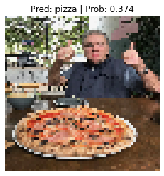 | | |